ANALYSIS OF VARIANCE
Analysis of variance (ANOVA) is a mathematical method of decomposing the total variation observed in an experiment into portions attributable to individual factors evaluated in the experiment. Another way of saying this is to say that ANOVA divides total process variation into segments based on different causal factors. The largest contributors are identified, based on a statistic called F. A more complete discussion will be given in Volume V of this series.
The purpose of using ANOVA is to quantitatively estimate the relative contribution that each factor has on the overall variation in the function of the product or process.
ANOVA, in conjunction with Taguchi's quality loss function (QLF), is used in tolerance design (TD) when the trade-off of quality and cost is at issue. To understand tolerance design, we must first understand the QLF.
By definition, QLF is a method that determines the economic loss per unit that the system renders because of its inherent performance; in other words, variation in performance. The QLF provides a quantitative estimate of the average monetary loss incurred by "society" (i.e., the manufacturer and consumer), when performance deviates from its intended target value.
ANOVA is used in problem solving and, in particular, TD to determine the significance of each factor for the system performance, whereas QLF is used to determine the monetary impact of each factor on the system performance. This is truly remarkable knowledge because once this fact is known and the cost of upgrading is identified, an engineer can make rational decisions regarding the quality versus cost trade-off.
The following are the steps for conducting TD:
Step 1. Conduct the experiment.
-
Preparation; efficient and successful experiments require knowledge regarding the following:
-
System function
-
Output response to be optimized
-
Target value for output response
-
Tolerance for output response
-
Cost for quality improvement when output response is out of specification
-
Potential tolerance factors and levels which contribute to system variation
-
Cost for upgrading or tightening the tolerances
-
-
Orthogonal arrays ”Once the tolerance factors and their levels are determined, they are assigned to an appropriate orthogonal array (OA). Although there are many OAs to choose from, the L 12 is suggested for manufacturing; the L 18 for design; and the L 36, as well as the L 54 , for computer simulation. More will be discussed about OAs in Volume V of this series. Other OAs may be used if interactions are to be evaluated.
Step 2. Perform ANOVA analysis ”Once data are collected for each trial in the OA, analysis begins using ANOVA. A typical ANOVA output is shown in Table 2.9.
| Source | df | SS | Variance | SS' (Pure Sum of Squares) | (rho; %) |
|---|---|---|---|---|---|
| Factor A | |||||
| Factor B | |||||
| . | |||||
| . | |||||
| . | |||||
| Factor N | |||||
| Error | |||||
| Total |
-
Sum of squares (SS): Quantifies the deviation of each effect value from the overall mean value. Sum of squares for factor P :
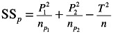 or
or SS p = [r(effect) 2 ]/number of levels for factor
where
T
=
total of all data
T 2 ln
=
correction factor
P i
=
sum of data under P i condition
n P l
=
number of data points under the P i condition
r
=
number of responses/number of levels of each factor
Of course, total variability of the system is

-
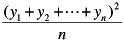
Sum of squares for total:
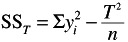 or
or 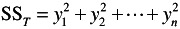
where
T 2 /n
=
CF = correction factor =
n
=
number of responses
y
=
the actual response
n - 1
=
degrees of freedom
-
Variance ( V ): Quantifies the mean value of the sum of squares for each effect by dividing by the degrees of freedom associated with the effect.
-
Variance for factor P is
V p = SS P /df p
-
Variance for total is
V Total = SS Total /df Total
Of note here is the fact that if only one repetition is collected for each trial, and all columns of the OA are used to evaluate factor effects, V error (variance due to error) cannot be computed, as SS error and df error will be equal to 0.
V error = SS error /df error
-
A technique called pooling is often used to obtain an estimate of error variance, V error . (It must be mentioned, however, that if columns are left empty or there are repetitions, error can be estimated with or without pooling.) Pooling in essence amounts to adding relatively small sum of squares values together to simulate an error term . The actual process involves two-steps:
-
Calculate the percentage contribution ( -rho) for each factor.
-
Pool all sums of squares whose percentage contribution value is relatively small compared with the sum of squares value for other factors
In conjunction with pooling, there is also the SS' (pure sum of squares), which quantifies the magnitude of each effect when the error variance ( V error ) is subtracted.
-
Pure SS for factor P =
 = SS P - (df P )( V error )
 -
Pure SS for total =
 = SS Total
 -
Pure SS for error =
 = SS error + (df Total - df error )( V error ) =
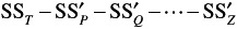
To actually calculate these values, we use the following formulas (percentage contribution quantifies the relative percentage contribution that each effect has on the total variation observed in the experiment):
-
Percentage contribution for factor P = p =
 — 100
— 100 -
Percentage contribution for Total = Total =
 — 100 ( ALWAYS equal to 100%)
 -
Percentage contribution for error = error =
 — 100
— 100
-
GLOBAL PROBLEM-SOLVING PROCESS
In Volume II of this series, we spent much time and effort to describe this process in detail. Here we give a cursory review by defining the goals and expectations of each of the eight steps.
-
Use a team approach. Organize a group of people who have the necessary
-
time,
-
knowledge of the product and process,
-
authority and responsibility, and
-
technical knowledge.
Team members may include nonproduction personnel. Choose a leader who organizes and drives the improvement process.
-
-
Describe the problem. The first step is to illustrate the actual (manufacturing, service, etc) process. Use a process flow chart to identify where the problem is observed and where it originates. Identify places where the process can be sampled.
As a team, brainstorm ideas about causal factors. Use a cause and effect (fishbone) diagram to organize these ideas. Define the problem in measurable terms. Use a Pareto chart to measure the size of the problem. To determine when the problem occurs, examine the process log and use a control chart, if available.
-
Implement and verify interim (containment) actions. Plan and carry out steps to quarantine the problem and its results. Protect the customer from receiving nonconforming parts . Team members should consult customer control charts and Pareto charts to make sure that the problem has been contained.
-
Define and verify root causes. True problem solving means eliminating and preventing the root causes of a problem rather than reacting to symptoms. As a team, construct cause and effect (fishbone) diagrams for the problem. Use the diagrams to record theories that the team should test with experiments and distribution analyses. When satisfied that the causal factors have been found, plan and implement corrective actions.
-
Verify corrective actions. Sample the process before and after making corrections. The data should verify the effectiveness of the action. The team should run experiments, analyze distributions, and use control charts to plot data from before and after the correction. Ask the customer if the corrective action solved the customer's concerns. Make sure that the corrective action did not cause other or similar problems.
-
Implement permanent corrective action. If the corrective action is effective, make it a permanent part of the process. Use ongoing control charts to study the long-term effectiveness of the solution.
-
Prevent recurrence . Use the team's theories from the definition and verification step to completely avoid experiencing the problem again. This requires acting on process elements before they create problems.
-
Congratulate your team. Improvements are achieved only through the efforts of many people working together. Recognize and congratulate all contributors.
STATISTICAL PROCESS CONTROL
As we have already suggested, SPC is a method for determining the cause of variation based on statistical analysis of the problem. SPC uses probability theory to control and improve processes. Fundamentally, SPC does two things:
-
Identifies problems in the process
-
Identifies the type of variation in the process
-
common variation is the random happenings in the process
-
special variation is the abnormalities in the process
-
It has been empirically found that SPC is indeed an effective methodology for problem solving and for improving performance of any process. It helps identify problems quickly and accurately. It also provides quantifiable data analysis, provides a reference baseline, and promotes participation and decision making by people closest to the job.
What is the process of SPC? Fundamentally, the process of doing SPC in any activity is to:
-
Identify problems or performance improvement areas and identify common and special causes. Common causes are random in nature, often minor. Special causes result from an abnormality in the system that prevents the process from becoming stable.
-
Do a cause and effect analysis
-
Collect data
-
Apply statistical techniques (in some cases, a statistical specialist is needed)
-
Analyze variation
-
Take corrective action
Implementing Process Control System
Most people think that the essence of SPC is to generate "some" charts and then relax. That is the furthest from the truth. Problem solving is a continual issue of improvement. Once you can do the charts, if that is appropriate and applicable for the situation, applying the information can sometimes be more difficult. There are four underlying assumptions to solving process control problems:
-
The effort must be a team effort. This is better than a coordinated or individual effort.
-
When problems are identified, the right action must take place at the right time.
-
Fixed problems must be stopped from happening again by constant monitoring and feedback.
-
The effort must be one of clearly defining assignable variation. It is not of assigning blame.
Burr (1976) identified several steps in solving control problems. We list them here.
-
The problem naturally involves some product or material that is not satisfactory. Determine what quality characteristic is causing the most trouble.
-
When there is a suitable measuring tool for the feature in question, test it. Make sure it gives repeatable results. The same piece, measured twice, should give the same results each time.
-
Sometimes, no measuring tool exists, and it may be best to make one. Variables measurement control charts are more efficient at finding trouble than are attribute charts.
-
When using attribute charts, clearly define a defect or defective unit. This can be checked as in #2 above. A larger number of samples or pieces should be offered for attribute inspection.
-
Get at the beginning of the problem. Go back to the operations on the product. Find out where the trouble first began (for example, in machining or grinding operations, it is often the first rough work). Samples should be drawn as near to that operation as possible. The testing or measurement should be done as soon as possible after the operation is performed.
-
Make a list (brainstorm) of the likely special causes that need to be corrected. Talk to everyone connected to the operation. The operator, setup man, inspector, foreman, engineer, designer, chemist, or whoever may have some ideas on it.
-
There may be some useful data already available. Usually, this is not the case. Results may not be in a useful sample size. Conditions were not adequately controlled. A record was not made of the condition under which the pieces were made and tested . Attribute data more often are of use; it is worth looking for past data ”then there can be a comparison.
-
Arrange for the collection of new data. This involves the choice of sample size. Four or five pieces measured are standard. For a p-chart, sample size (n) can be small, but do not let the np go below 5. The same person should do the testing or measuring on the same test set; this way, any out-of-control signs are due to product variation and not to testing or personnel.
-
Careful record should be made of the conditions under which each sample was made. Record conditions on as many likely special causes (see #6) as possible. It is hard to record them all.
-
If old data are not on hand, then a new run of data must be collected. This is done by taking samples about as often as they can be handled. A quicker start can be made, and it is also often helpful to see how a run of most of the pieces behaves.
-
Study the beginning data. Show them to all people involved. Explain with great care and simplicity what the charts mean.
-
The hunt for special causes is now on. This is where teamwork counts. What conditions or likely special causes were different for the out-of-control conditions? Was there any one condition present for all the points out on the high side? Was this one condition not present on many, if any, of the other points? Were there any trends? Be sure that any resettings or retooling is marked on the chart. If the process is in control and still not meeting specs , a major change in the process will be required.
-
Corrective action must be tried on any suspected special cause. If no points go out for a while, test the process. Bring in the special cause again. See if any points go out or not. Finding and providing a special cause is an experimental job. The SPC facilitator can help you here.
-
Corrective action on a proven special cause may require action by management. It may also require spending money. The surest way to kill off a promising quality program is for management to repeatedly fail to take action when it is clearly needed or when it is economically sound.
-
A brief, clear, and factual report should go to the right person in the organization. Interesting graphs help. Money saved is always of interest to management. Also important is improved quality assurance.
-
Follow-through is basic. Control charts should be maintained even after the problem is completely solved. The samples may be taken at longer time intervals. They can still give warning when the process is getting out of hand. This is especially true when 100% sorting has been replaced by sampling. Operations have a tendency to get out of hand when not kept track of.
OTHER PROBLEM-SOLVING TECHNIQUES
As we discussed in Volume II, there are many ways to solve a problem, and many approaches have already been addressed. To review, we list some of these useful techniques below.
Regression Analysis
Used to optimize a process setup, regression analysis estimates process parameters and predicts outputs. Sometimes, as part of the regression analysis, subanalyses are performed such as correlation, scatter plot analysis, residual analysis, and many more.
Design of Experiments
Experimental designs establish plans for experiments and data analysis. Well-designed experiments are very efficient; they generate a great deal of information from a minimum of data. ANOVA is only one of the many ways to do experimentation. Design of experiments (DOE) is a collective approach of statistical analysis that is used to improve the process learning from experimentation. This learning enables improved process design.
The reason that we want to do a DOE is to improve the design-to-production transition. DOE optimizes product designs (robust design) and production processes. It reduces cost, stabilizes production processes, and desensitizes production variables.
To do a successful DOE, we must do the following:
-
Identify controllable and uncontrollable (noise) factors that influence the product's functional characteristics.
-
Set up an experiment to discover interactions and effects between controllable and uncontrollable factors.
-
Study the factor variation in Step 2 and determine the factor levels that optimize the product's functional characteristics, while minimizing the influence of uncontrollable factors.
Simulation Methods
Computer-based models are built to forecast the performance of a system before it is built.
EAN: 2147483647
Pages: 181