DEFINITION OF MEASUREMENT ERROR TERMS

One of the objectives of a measurement system study is to obtain information relative to the amount and types of measurement variation associated with a measurement system when it interacts with its environment. This information is valuable because for the average process, it is far more practical to recognize repeatability and calibration bias and to establish reasonable limits for these than it is to provide extremely accurate gages with very high repeatability . Applications of such a study provide the following:

• A criterion for accepting new measuring equipment

• A comparison of one measuring device against another

• A basis for evaluating a gage suspected of being deficient

• A comparison for measuring equipment before and after repair

• A required component for calculating process variation and the acceptability level for a production process

• Information necessary for development of a gage performance curve (GPC), which indicates the probability of accepting a part of some true value

To appreciate this process, we provide the reader with some basic definitions and graphical representations for the key concepts of the measurement system analysis.

• Uniformity is the difference in variation throughout the measurement range of the gauge. It is repeatability over time.

• Sensitivity is the least increment in the measured dimension that produces a usable, rather than a discernible, change on the instrument.

• Discrimination is the smallest graduation on the scale of the instrument. The rule is that the measuring equipment should be able to measure at least 1/10 of the process variation. The best indication of inadequate discrimination is given by the range chart. This is also known as readability.

• True value refers to the theoretically correct value of the characteristic being measured (Western Electric, 1977; Speitel, 1982). This theoretically correct number is the absolutely correct description of the measured characteristic. This is the value that is estimated each time that a measurement is made. The true value is never known in practice because of the measurement scale resolution or the divisions that are used for the instrument's output. An analyst may be perfectly satisfied with measuring the outside diameter of a shaft to thousandths of an inch (0.525 in.). A closer approximation to the true value is made when another instrument is represented with five decimal places (0.52496 in.). The appropriate level of measurement resolution is determined by the characteristic specifications and economic considerations. A common guideline calls for tester resolution that is equal to or less than 1/10 of the characteristic tolerance (USL - LSL). The true value is considered as part of tester calibration and discussions of measurement accuracy. Examples of true value (or known standard) devices include Jo-blocks and certain oscillators of known frequencies. These are the primary standards for the subject of the measurement.

• Precision is the extent to which the device provides repetitive measures on a single standard unit of product (Juran and Gryna, 1980). That is, it is a measure of the degree of agreement among individual measures on a given standard sample (Speitel, 1982). Usually, the distribution of these measures may be approximated by the normal distribution (Juran and Gryna, 1980; Speitel, 1982; Western Electric, 1977). Further, precision is typically assessed in the context of prescribed and uniform (similar) conditions. The degree of precision in a measurement process is generally designated as the standard deviation of measurement error, or ƒ _E (Juran and Gryna, 1980; Speitel, 1982; Western Electric, 1977). The common variation contributing to the precision of the measurement process generally originates in two domains: variation due to repeatability and variation due to reproducibility (Speidel, 1982). Because repeatability and reproducibility are quantified as parts of the standard deviation for measurement error, some people call measurement error analyses "R & R studies."

• Repeatability is generally used to define precision estimates for a limited set of specifically defined conditions; that is, the variability in individual measures over the same parts for one gage or operator or system, at one time (Speitel, 1982). Another way of defining repeatability is the variation in measurements obtained with one measurement instrument when used several times by one appraiser while measuring the identical characteristic on the same part (AIAG, 1995, 2002). This can be shown in Figure 15.3. Both figures show the same thing but from a different perspective. Both show the differences in successive measured readings for one part, made by one person, using one instrument, in one setting or environment, using one calibration of reference as error due to repeatability. This is the variation within a situation or scenario. Repeatability is present in every measurement system. However, Figure 15.3a shows the entire variation of the measurement, whereas Figure 15.3b shows a distribution of repeated measurements that were made on one part, by one person, with one tester. The mean of the curve is not located near the true value for the part. This indicates the inaccuracy of the measurement system. The instrument should be recalibrated. The spread of the curve illustrates the degree of error due to repeatability. The calculated deviation for this distribution quantifies the level of repeatability error.

  
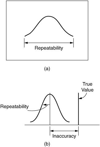
  Figure 15.3: Repeatability.

• Reproducibility, on the other hand, is the variability in measures of sample parts that is due to differences between gages or operators or systems and (for the purpose of this chapter) relates to that variability for a (relatively) short time period under a set of specific conditions. Another way of saying this is that reproducibility is the variation in the average of the measurements made by different appraisers, using the same measuring instrument when measuring the identical characteristic on the same part (AIAG, 1995, 2002).

Reproducibility describes the difference in successive measurements for the same part that is due to differences between hardware, people, methods , or environments. This source of variability is quantified as the spread (range or standard deviation) between the means of several repeatability distribution (see Figure 15.4). Figure 15.4a shows a reproducibility situation with three operators; Figure 15.4b shows the general rule of reproducibility when there is more than one measurement situation. Because three different people use the same testers to setup a machining center, three setup people were asked to create repeatability distributions by measuring the same part a number of times. The results of the measurements are shown in Figure 15.4b. None of the people had perfect accuracy. Persons B and C were closer to the true value than was Person A. Each of the repeatability curves had a similar magnitude of spread. This means that each of the people had nearly the same degree of repeatability error within their measurement techniques. Reproducibility is the distance between the means, or the measurements of Persons A and C. This difference shows the amount of measurement error among the three people.

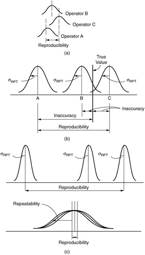
Figure 15.4: Reproducibility.

A study that quantifies repeatability and reproducibility contains much diagnostic information. This information should be used to focus measurement system improvement efforts. Graphic illustrations of the information help people understand the results of the studies (see Figure 15.4c). The curves in Figure 15.4c show three repeatability distributions. Error due to repeatability is smaller than the error due to reproducibility. Although each situation contains relatively small amounts of repeatability error, there is a large difference between each of the measurement activities. This is typical when people use different calibration or measurement methods.

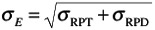
The distributions in Figure 15.4c have means that are almost equal. This indicates a very small degree of reproducibility error. The error that is inherent in each measurement situation is very large. In this case, all of the measurement activities are using the same calibration and measurement procedures. Despite these similarities, all of the distributions experience a high degree of repeatability error. This signals that there is a source of error that is common to each of the measurement situations. The measurement hardware or anything else that is common to each of the distributions should be investigated as a major source of measurement error. The ƒ _E , therefore, is a compilation of variability due to repeatability ( ƒ _RPT ) and reproducibility ( ƒ _RPD ), and it may be evaluated as

In those cases in which only one gage or operator or system is involved, the short- term precision of the measurement process is described solely by the variability of the repeatability domain, so that

ƒ _E = ƒ _RPT

• Stability (or drift ) is the total variation in the measurements obtained with a measurement system on the same master or parts when measuring a single characteristic over an extended time period (see Figure 15.5).

  
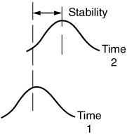
  Figure 15.5: Stability.

A different way of looking at stability is to think of it as a measure of the dependability , or consistency, of the measurement process over time (i.e., long term). For the purpose of this chapter, stability may be thought of in terms of changes in the precision of the measurement process over time due to the effects of changes in the sources of variation affecting the process. The additional time period allows additional opportunity for the sources of repeatability and reproducibility error to change and add error to the measurement system. All measuring systems should be able to demonstrate stability over time. A control chart made from repeated measurements of the same parts documents the level of a measurement system's stability. Furthermore, the addition of the aspect of stability to measurement error ( related to precision, not accuracy) would generally have the effect of adding variability to the ƒ _E due to repeatability and reproducibility (if present) of the measurement process. It may be helpful to think of these aspects in the context of capability studies commonly conducted for production equipment. A machine capability study is a measurement device analysis of ƒ _E due to repeatability and reproducibility; process capability is analysis of ƒ _E due to repeatability, reproducibility, and stability.

Of course, that description is presented for analogy purposes. The association of machine capability with short-term studies and of process capability with long-term studies should not be interpreted as an indication that machine capability studies are always short-term in nature. In point of fact, machine capability analyses may be conducted over a short or long period of time.

• Accuracy is the extent to which the average (Xbar) of a long series of repetitive measurements made by the instruments on a single unit or product differs from the true value of the product (Juran and Gryna, 1980; Western Electric, 1977). An instrument or measurement process with an Xbar measurement value that is different from the product's true value because of bias is said to be "out of calibration" (Juran and Gryna, 1980). This distinction may be seen in Figure 15.6.

  
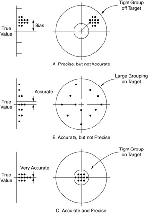
  Figure 15.6: The distinction between precision and accuracy.

Figure 15.6 shows the similarity between target practice and the measurement error concepts of precision and accuracy. The center of the target represents the true value of a measured characteristic. When the group of shots is centered around the true value, the measurement system is accurate. Figures 15.6B and 15.6C are accurate because the centers of the groups are very close to the center of the target. The histograms to the left of the targets summarize the vertical distance of each shot from the center of the target. The means for Figures 15.6B and 15.6C are almost directly on top of the true values. The illustration in Figure 15.6A shows a group of shots that is not centered. This would translate to a measurement system that is not accurate. This measurement system requires calibration so that it becomes like the distribution in Figure 15.6C.

The spread of the shots describes the precision of the measurement process. A tight group indicates precision (see Figures 15.6A and C). A broad spread means that the error or lack of precision is high. Although the center of the distribution in Figure 15.6B is centered (it is accurate), the measurement system has much error because of lack of precision. This form of error will not be reduced with additional calibration. This measurement system has already been calibrated properly, and additional adjustment will only make it less accurate.

• Bias is the difference between the observed average of measurements and the reference value. The reference value, also known as the accepted reference value or master value , serves as an agreed-upon reference for the measured values. A reference value can be determined by averaging several measurements with a higher level of measuring equipment. Bias is also known as accuracy (AIAG, 1995, 2002). This can be seen in Figure 15.7.

  
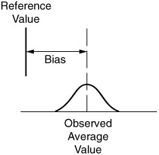
  Figure 15.7: Bias.

  If the bias is relatively large, look for these possible causes:

  • Worn components

  • Instrument used improperly by appraiser

  • Instrument not calibrated properly

  • Instrument made to the wrong dimensions

  • Error in the master

  • Instrument measuring the wrong characteristic

• Linearity is the difference in the bias values through the expected operating range of the gage (see Figure 15.8). Figure 15.8a shows the range of the bias, whereas Figure 15.8b shows the relationship of bias and no bias in linearity terms.

  
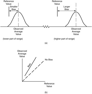
  Figure 15.8: Linearity.

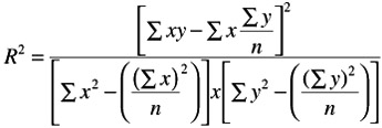
The goodness of fit can be used to make an inference about the linear association between the bias and reference value. From this, we can conclude whether there is a linear relationship between them and, if so, whether it is acceptable. It must be reemphasized, however, that linearity is determined by the slope of the line of best fit and not by the goodness-of-fit ( R ² ) value for the line. Generally, the lower the slope, the better the gage linearity, and conversely, the greater the slope, the worse the gage linearity.

Note  

Although the R ² value is one of the most frequently quoted values from a regression analysis, it does have one serious drawback. It can only increase when extra explanatory variables are added to an equation. This can lead to " fishing expeditions," in which we keep adding variables to an equation, some of which have no conceptual relationship to the response variable, just to inflate the R ² value. To penalize the addition of extra variables that do not really belong, an adjusted R ² (Adj R ² ) value is typically listed in regression outputs. Although it has no direct interpretation as percentage of variation explained, it can decrease when extra explanatory variables that do not really belong are added to an equation.

Therefore, the R ² is a useful index that we can monitor in our analysis, especially if a computer software package is used. If we add variables and the adjusted R ² decreases, then we know that the extra variables do not pull their own weight and probably should be omitted.

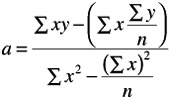
In the simplest form, linearity may be computed as a linear equation:

y = a + bx

where

x	=	reference value
y	=	bias
a	=	slope

• Error of measurement , as shown by the previous illustrations, may be discussed in the context of error in the precision of the measurement process (the thrust of this chapter) and in terms of the bias affecting the accuracy of the measurement process.

As previously described, the short-term precision error (or measure-to-measure variability) is a function of error due to repeatability, reproducibility, or both. Bias, on the other hand, affects (largely) the accuracy of the measurement process and is a function of either constant or variable errors. Constant errors affect all measurements by the same amount and are generally associated with problematic setup procedures, such as inaccurate standards, poor alignment, or incorrect conversion factors. An example of this source of error would be a dial indicator that was "zeroed out" at 0.002 to the minus side. As a result (not considering precision variability), the average of all measures would be affected by 0.002 to the negative side.

Variable errors, on the other hand, display changes in magnitude within the range of the measurement process or scale. These errors are frequently related to the construction of the measuring equipment itself. An example of this type of error is a steel rule with uniform but too-tight graduations. In this case, the magnitude of error would be proportional to the size of the product measured. Another example would be power supply voltage to a gaging head that varies with line voltage causing a variable biasing of the gage head.

• Standard deviation of measurement error concerns the spread of the precision distribution, which is calculated as a composite because precision is separated into the domains of repeatability and reproducibility. The standard deviation for measurement error is calculated as

  

  Six standard deviations of measurement error describe the spread of the precision distribution. The magnitude of this spread is evaluated with the precision/tolerance (P/T) ratio.

• Measurement gauge capability ”is determined by the variability of the measures produced. For a measurement process to be capable, the variability of the measures (i.e., the precision distribution, as measured by ƒ _E ) must not account for a significant portion of the specification or tolerance window for the unit or product (Charbonneau and Webster, 1978). As with machine and process capability, measurement capability requirements vary based on whether the analysis is a short-term or long-term study.

  For the purposes of this chapter, therefore, a capable gage or measurement process will be one in which the following are true (Charbonneau and Webster, 1978; Juran and Gryna, 1980; Speitel, 1982):

  • The short-term P/T ratio is less than .10.

  • The long-term P/T ratio is less than .25.

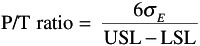
• PIT ratio ”value is the ratio between the measurement precision estimate and the tolerance (difference between the minimum and maximum limits) of the characteristic being measured. A measurement system is declared adequate when the magnitude of measurement error is not too large. One way to evaluate the spread of the precision distribution is to compare it with the product tolerance. This is an absolute index of measurement error because the product specifications should not change. A measurement system is acceptable if it is stable and does not consume a major portion of the product tolerance. The ratio between the precision distribution (6 standard deviations of measurement error) and the product tolerance (upper and lower specification limits) is called the P/T ratio and quantifies this relationship.

  

where

ƒ E	=	standard deviation of measurement error
USL	=	upper specification limit
LSL	=	lower specification limit

The above formula may also be written as

P/T ratio = 6 ƒ _E /total tolerance

It is important to note that this ratio is based on the following assumptions:

• Measurement errors are independent.

• Measurement errors are normally distributed.

• Measurement error is independent of part size.

• For normal distributions with bilateral specifications, the total tolerance is the specification range, or window (i.e., USL - LSL). For normal distributions with a unilateral specification, the total tolerance may be estimated as

  

where

Xdouble bar	=	mean of process
SL	=	upper or lower specification limit

Further, the assessment of measurement capability is predicated on the assumption that the sources of accuracy error will be removed or eliminated, which has the effect of centering the precision distribution on the nominal or target value (i.e., true value of the part or parts).

The primary use and application of the measurement capability analysis is in the evaluation of the effects of error on the acceptance and rejection decisions, as conducted for individual parts. This relationship is reflected in Figure 15.9 and is discussed in depth by Eagle (1954).

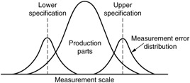
Figure 15.9: The relationship of error and acceptance.

The following general criteria are used to evaluate the size of the precision distribution:

P/T Ratio Level of Measurement Error
0 “.10	Excellent
.11 “.20	Good
.21 “.30	Marginal
.31+	Unacceptable