ANALYSIS OF CLASSIFIED DATA

The purpose of this section is to:

Discuss the classified attribute analysis and classified variable analysis approaches to analyzing classified responses.
Present examples of how these techniques are used.

CLASSIFIED RESPONSES

Some experimental responses cannot be measured on a continuous scale although they can be divided into sequential classes. Examples include appearance and performance ratings. In these situations, three to five rating classes are generally the optimum number because this number allows major differences in the responses to be identified and yet does not require the rater to identify differences that are too subtle. Two related techniques are used to analyze classified responses:

Classified attribute analysis is used when the total number of items rated is the same for every test matrix setup.
Classified variable analysis is used when the total number of items rated is not the same for every test matrix setup.

Three to five responses at each experimental setup are recommended to give a good evaluation of the class distribution of responses at that setup. As with continuous measurements, more responses at each setup allow smaller differences to be identified.

CLASSIFIED ATTRIBUTE ANALYSIS

This technique converts the observed frequency in each class into a cumulative frequency for the classes. As an example, if there are three classes, the observed and cumulative frequencies might be as shown in Table 9.33.

Table 9.33: Observed Versus Cumulative Frequency
	Observed Frequency	Cumulative Frequency
Class I	2	2
Class II	1	3
Class III	1	4

It is assumed that the user will use a computer program to analyze the classified data. The specific input format will depend on the computer program used. The mathematical derivations and philosophies of this approach will not be presented here. For more information see Volume V of this series as well as Taguchi (1987) and Wu and Moore (1985).

Three grades are used to evaluate paint appearance of a product. They are "Bad," "OK," and "Good." Seven factors (A through G), each at two levels, are evaluated to determine the combination of factor levels that optimizes paint appearance. Five products are evaluated at each testing situation in an L8 orthogonal array. Test results are shown in Table 9.34.

Table 9.34: Attribute Test Setup and Results
							Frequency in Each Grade
A	B	C	D	E	F	C	Bad	OK	Good
1	1	1	1	1	1	1	2	3
1	1	1	2	2	2	2	3	2
1	2	2	1	1	2	2	4	1
1	2	2	2	2	1	1		2	3
2	1	2	1	2	1	2		4	1
2	1	2	2	1	2	1	1	3	1
2	2	1	1	2	2	1		3	2
2	2	1	2	1	1	2		1	4

The ANOVA analysis for this set of data is shown in Table 9.35. Note that the degrees of freedom are calculated differently from the non-classified situation. The df of each source is:

(the number of levels of that factor - 1) * (the number of classes - 1)

Table 9.35: ANOVA Table (for Cumulative Frequency)
Source	df	SS	MS	F Ratio	S'	%
A	2	11.668	5.834	7.820	10.179	12.72
B	2	6.678	3.39	4.476	5.186	6.48
C	2*	0.125	0.063
D	2*	3.668	1.834
E	2*	2.259	1.130
F	2	7.935	3.986	5.319	6.443	8.05
G	2*	2.259	1.130
Error	64	45.409	0.710
(pooled error)	72	53.720	0.746		58.196	72.75
Total	78	80.000	1.026

In this example, the number of levels of each factor is two and the number of classes is three. For each factor,

The total df = (the total number of rated items - 1) * (the number of classes - 1). Thus, the total df for this example is:

The error df is the total df minus the df of each of the factors.

From the ANOVA table, factors A, B, and F are identified as significant. The effects of these factors are shown in Table 9.36 and Figure 9.21.

Table 9.36: The Effect of the Significant Factors
	Observed Frequency			% Rate of Occurrence (R.O.)			Cumulative Frequency			Cumulative % R.O.
	Bad	OK	Good	Bad	OK	Good	Bad	OK	Good	Bad	OK	Good
A1	9	8	3	45	40	15	9	17	20	45	85	100
A2	1	11	8	5	55	40	1	12	20	5	60	100
B1	6	12	2	30	60	10	6	18	20	30	90	100
B2	4	7	9	20	35	45	4	11	20	20	55	100
F1	2	10	8	10	50	40	2	12	20	10	60	100
F2	8	9	3	40	45	15	8	17	20	40	85	100
Total	10	19	11							25	73	100

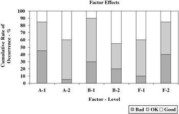
Figure 9.21: Factor effects.

Although interpretation and use of the ANOVA table in classified attribute analysis is the same as for the non-classified situation, a significant difference does exist in estimating the cumulative rate of occurrence for each class under the optimum condition.

Percentages near 0% or 100% are not additive. The cumulative of occurrence can be transformed using the omega method to obtain values that are additive. In the omega method, the cumulative percentage (p) is transformed to a new value ( ) as follows :

= -10 log ₁₀ [the units of are decibels (db).]

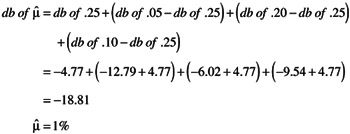
Using this transformation, the estimated cumulative rate of occurrence for each class at the optimum condition (A ₂ B ₂ F ₁ ) is calculated as follows:

The estimated cumulative rate of occurrence for each class for the optimum condition is:

Class 1

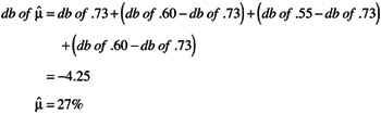
Class 2

These results are summarized in Table 9.37.

Table 9.37: Rate of Occurrence at the Optimum Settings
Class	Cumulative Rate of Occurrence	Rate of Occurrence
Bad	1%	1%
OK	27%	26%
Good	100%	73%

CLASSIFIED VARIABLE ANALYSIS

Classified variable analysis is used when the number of items evaluated is not the same for all test matrix setups. As with classified attribute analysis, the computer analyzes the cumulative frequencies.

Four factors (A, B, C and D) are suspected of influencing door closing efforts for a particular car model. An experiment was set up that evaluated each of these factors at three levels. An L9 orthogonal array was used to evaluate the factor levels. Door closing effort ratings were made by a group of typical customers. Each customer was asked to evaluate the doors on a scale of one to three as follows:

Class	Description of Effort
1	Unacceptable
2	Barely acceptable
3	Very good feel

The experimental setup and test results are shown in Table 9.38 and Figure 9.22. The ANOVA analysis for this set of data is shown in Table 9.39.

Table 9.38: Door Closing Effort: Test Setup and Results
A	B	C	D	Number of Ratings	Ratings by Class			Class% Rate of Occurrence			Class Cumulative Frequency (%)
A	B	C	D	Number of Ratings	1	2	3	1	2	3	1	2	3
1	1	1	1	5	1	3	1	20	60	20	20	80	100
1	2	2	2	4	2	1	1	50	25	25	50	75	100
1	3	3	3	5	2	3		40	60		40	100	100
2	1	2	3	4			4			100			100
2	2	3	1	4		1	3		25	75		25	100
2	3	1	2	4		1	3		25	75		25	100
3	1	3	2	5	3	2		60	40		60	100	100
3	2	1	3	5	4	1		80	20		80	100	100
3	3	2	1	4	3	1		75	25		75	100	100

Table 9.39: ANOVA Table for Door Closing Effort
Source	df	SS	MS	F Ratio	S'	%
A	4	871.296	217.824	447.277	869.348	48.30
B	4	34.404	8.601	17.661	32.456	1.80
C	4	25.125	6.296	12.928	23.234	1.29
D	4*	4.827	1.207
Error	1782	864.291	0.485
(pooled error)	1786	869.118	0.487		874.962	48.61
Total	1798	1800.000	1.001

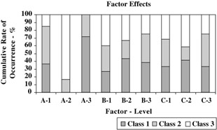
Figure 9.22: Factor effects.

From the ANOVA table, factors A, B and C are identified as significant. The effects of these factors are shown in Table 9.40.

Table 9.40: The Effects of the Door Closing Effort
Factor & Level	% Rate of Occurrence			Cumulative % Rate of Occurrence
Factor & Level	Class 1	Class 2	Class 3	Class 1	Class 2	Class 3
A1	36.7	48.3	15.0	36.7	85.0	100
A2		16.7	83.3		16.7	100
A3	71.7	28.3		71.7	100.0	100
B1	26.7	33.3	40.0	26.7	60.0	100
B2	43.3	23.3	33.3	43.3	66.6	100
B3	38.3	36.7	25.0	38.3	75.0	100
C1	33.3	35.0	31.7	33.3	68.3	100
C2	41.7	16.7	41.7	41.7	58.4	100
C3	33.3	41.7	25.0	33.3	75.0	100
Total	36.1	31.1	32.8	36.1	67.2	100

The choice of the optimum levels is clear for factors A and B. A ₂ and B ₁ are the best choices. Two different choices are possible for factor C, depending on the overall goal of the design. If the goal is to minimize the occurrence of unacceptable efforts, C ₁ is the best choice. If the goal is to maximize the number of customer ratings of "very good," then C ₂ is the best choice. For this example, C ₁ will be chosen as the preferred factor setting. The estimated rate of occurrence for each class for the optimum setting, A ₂ B ₁ C ₁ , can be calculated using the omega method. The estimated rates are shown in Table 9.41. The df for the factors are calculated in the same way as with the Classified Attribute Analysis, i.e., df = (the number of levels of that factor - 1) * (the number of classes - 1).

Table 9.41: Rate of Occurrence at the Optimum Settings
Class	Cumulative Rate of Occurrence	Rate of Occurrence
1 (unacceptable)	0%	0%
2 (barely acceptable)	13.4%	13.4%
3 (very good feel)	100%	86.6%

In Classified Variable Analysis, the total number of items evaluated at each condition is not equal. To "normalize" these sample sizes, percentages are analyzed and the "sample size " for each test setup becomes 100 (for 100%). The total df is (the number of "sample sizes" - 1) * (the number of classes - 1). For this example, the total df is:

The error df is the total df minus the df of each of the factors.

DISCUSSION OF THE DEGREES OF FREEDOM

In both classified attribute analysis and classified variable analysis, the total degrees of freedom are much greater than the number of items evaluated. The interpretation of the F ratios and the calculation of a confidence interval are complicated by the large number of degrees of freedom and will not be addressed here. The analysis techniques for classified responses are not as completely developed as are the techniques for the analysis of continuous data. In Dr. Taguchi's approach, the emphasis is on using the percent contribution to prioritize alternative choices. Although better statistical techniques may be developed to handle classified data, classified attribute and classified variable analyses can be used to identify the large contributors to variation in classified responses.

MISCELLANEOUS THOUGHTS

As we just mentioned in the discussion of the degrees of freedom, there is no consensus among statisticians regarding the best method to use to analyze classified data. A method that is an alternate to the ones described in this section is to transform the classified data into variable data and analyze the data as described in Section 5. A drawback to this approach is that the relative difference in the transformed values should reflect the relative difference in the classifications, and this is sometimes difficult to achieve. A simple example from the medical field will illustrate this. Four different groups of patients suffering from the same disease are each given a different medicine. The purpose is to determine which medicine is best. The response classes are shown in below:

Class	Description of Effect
A	Patient improves
B	No change in patient
C	Patient dies

If Class A is given a value of 1 and Class B is given a value of 2, what should Class C be given? Is the difference between Classes B and C the same as the difference between Classes A and B? Twice the difference? Three times?

Dr. George Box is of the opinion that this difficulty can be overcome by analyzing the variable data using several different transformations from the classifications. In most instances, the choice of the best response will not be affected by the different relative values placed on the classifications and, in every case, the data will be much easier to analyze and interpret. The example given earlier dealing with classified attribute data will be worked as an example.

Three grades are used to evaluate paint appearance of a product. They are "Bad," "OK," and "Good." The classified data are transformed into variable data as follows: Bad = 1; OK = 3; Good = 4. This puts emphasis on avoiding situations that result in "bad" responses. Seven factors (A through G), each at two levels, are evaluated to determine the combination of factor levels that optimizes paint appearance. Five products are evaluated at each testing situation in an L8 orthogonal array. Test results are shown in Table 9.42. The ANOVA analysis for the raw data is shown in Table 9.43. Plotting of the data and inspection of the level averages reveal that the best factor choices are: A ₂ B ₂ F ₁ . The ANOVA analysis for the NTB S/N ratios is shown in Table 9.44.

Table 9.42: OA and Test Setup and Results
Test Setup and Results
							Frequency in Each Grade
A	B	C	D	E	F	G	Bad	OK	Good	Transformed Data
1	1	1	1	1	1	1	2	3		1	1	3	3
1	1	1	2	2	2	2	3	2		1	1	1	3
1	2	2	1	1	2	2	4	1		1	1	1	3
1	2	2	2	2	1	1		2	3	3	3	4	4
2	1	2	1	2	1	2		4	1	3	3	3	4
2	1	2	2	1	2	1	1	3	1	1	3	3	4
2	2	1	1	2	2	1		3	2	3	3	3	4
2	2	1	2	1	1	2		1	4	3	4	4	4

Table 9.43: ANOVA for the Raw Data
Source	df	SS	MS	F Ratio	S'	%
A	1	11.03	11.03	14.33	10.26	20.94
B	1	3.03	3.03	3.93	2.26	4.61
C	1*	0.03	0.03
D	1*	2.03	2.03
E	1*	2.03	2.03
F	1	7.23	7.23	9.39	6.46	13.18
G	1*	2.03	2.03
Error	32	21.60	0.68
(pooled error)	36	27.70	0.77		30.01	61.27
Total	39	48.98	1.26

Table 9.44: ANOVA Table for the NTB S/N Ratios
Source	df	SS	MS	F Ratio	S'	%
A	1	23.81	23.81	16.76	22.39	25.18
B	1	23.81	23.81	16.76	22.39	25.18
C	1*	0.39	0.39
D	1*	0.39	0.39
E	1	13.21	13.21	9.29	11.79	13.26
F	1	23.81	23.81	16.76	22.39	25.18
G	1*	3.49	3.49
Error	3
(pooled error)		4.26	1.42		9.95	11.19
Total	7	88.91	12.70

Plotting of the S/N data and inspection of the level averages reveals that the best factor choices are: A ₂ B ₂ E ₂ F ₁ . The best choices overall are: A ₂ B ₂ E ₂ F ₁ . This compares with the best choice of A ₂ B ₂ F ₁ from the accumulation analysis on page 425.

Each of the methods has one further disadvantage . Using the transformation approach, it is not possible to make a projection of what the distribution of classes would look like at the optimum settings. The accumulation analysis was not able to identify the effect on the standard deviation of the ratings due to factor E. Each approach tells a different part of the story and both should be used to get the full picture.