SETTING UP THE EXPERIMENT

This section discusses:

1. The choice of the number of levels for each factor

2. Fitting a linear graph to the experiment

3. Special applications to reduce the number of tests

4. How to handle noise factors in an experiment

CHOICE OF THE NUMBER OF FACTOR LEVELS

To review:

• A factor is a unique component or characteristic about which a decision will be made.

A factor level is one of the choices of the factor to be evaluated (e.g., if the screw speed of a machine is the factor to be investigated, two factor levels might be 1200 and 1400 rpm).

Investigating a larger number of levels for a factor requires more tests than investigating a smaller number of levels. There is usually a trade-off required concerning the amount of information needed from the experiment to be very confident of the results and the time and resources available. If testing and material are cheap and time is available, evaluate many levels for each factor. Usually, this is not the case, and two or three levels for each factor are recommended. An exception to this occurs when the factor is non-continuous, and several levels are of interest. Examples of this type of factor include the evaluation of a number of suppliers, machines, or types of material. This situation will be discussed later in this section.

The first round of testing is usually designed to screen a large number of factors. To accomplish this in a small number of tests, two levels per factor are usually tested . The choice of the levels depends upon the question to be addressed. If the question is "Have we specified the right spec limits?" or "What happens to the response in the clear worst possible situation?" then the choice of what the levels should be clear.

A more complicated question to address is "How will the distribution in production affect the response?" As suppliers become capable of maintaining low variability about a target value, testing at the spec limits will not give a good answer to this question. There are at least two approaches that can be used:

1. Test at the production limits, as a worst case.

2. Test at other points that put less emphasis on the tails of the distribution where few parts are produced and more emphasis on the bulk of the distribution. It is a difficult choice to pick two points to represent an entire distribution. If this approach is being used, a rule of thumb is to choose a level that encompasses approximately 70% of that distribution (mean ± 1 standard deviation).

The main point of this discussion is that the choice of levels is an integral part of the experimental definition and should be carefully considered by the group setting up the experiment.

The second and subsequent rounds of testing are usually designed to investigate particular factors in more detail. Generally , three levels per factor are recommended. Using two levels allows the estimation of a linear trend between the points tested. The testing of three levels gives an indication of non-linearity of the response across the levels tested. This non- linearity can be used in determining specification limits to optimize the response. Although this concept will be explored in more detail in a later section on tolerance design, its application can be illustrated as follows :

• First round of testing ” Level B of factor 1 gives a response that is more desirable than that given by level A. See Figure 9.7.

  
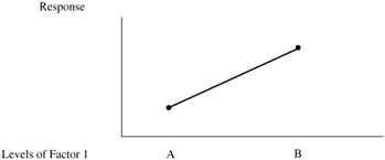
  Figure 9.7: First round testing.

• Second round of testing ” Level B gives a response that is more desirable than those given by either C or D. However, the differences are not great. Spec limits are set at C and D with B as the nominal. See Figure 9.8.

  
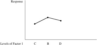
  Figure 9.8: Second round testing.

In a manner similar to the two-level -per-factor situation, the choice of the specific three levels to be tested depends upon the question under investigation. Testing at three levels can be used by the experimenter to focus on a particular area of the possible factor settings to optimize the response over as large a range as possible. If three levels of a factor are used to gain understanding for an entire distribution, a rule of thumb is to choose the levels at the mean and mean ± 1.225 standard deviations that encompass approximately 78% of the distribution. These rules of thumb will be used in tolerance design.

LINEAR GRAPHS

After the number of levels has been determined for each factor, the next step is to decide which experimental setup to use. Dr. Taguchi uses a tool called "linear graphs" to aid the experimenter in this process. Linear graphs are provided in the Appendix of Volume V for several situations. Typical designs, however, are:

1. All factors at two levels (L4, L8, L12, L16, L32)

2. All factors at three levels (L9, L27)

3. A mix of two- and three-level factors (L18, L36)

DEGREES OF FREEDOM

In the orthogonal array designation, the number following the L indicates how many testing setups are involved. This number is also one more than the degrees of freedom available in the setup. Degrees of freedom are the number of pair-wise comparisons that can be made. In comparing the levels of a two-level factor, one comparison is made and one degree of freedom is expended. For a three-level factor, two comparisons are made as follows: first, compare A and B, then compare whichever is "best" with C to determine which of the three is "best." Two degrees of freedom are expended in this comparison. Once the number of levels for each factor is determined, the degrees of freedom required for each factor are summed. This sum plus one becomes the bottom limit to the orthogonal array choice.

The degrees of freedom for an interaction are determined by multiplying the degrees of freedom for the factors involved in the interaction.

• A two-level factor interacting with a two-level factor requires one degree of freedom (df) (1 — 1 = 1).

• A three-level factor interacting with a three-level factor requires 4 df (2 — 2 = 4).

• A three-level factor interacting with a two-level factor requires 2 df (2 — 1 = 2).

Although the test response should be chosen to minimize the occurrence of interactions, there will be times when the experts know or strongly suspect that interactions occur. In these cases, linear graphs allow the interaction to be readily included in the experiment.

If more than one test is run for each test setup, the total df is the total number of tests run minus one. The dfs used for assigning factors remain the same as without the repetition. The other dfs are used to estimate the non- repeatability of the experiment.

USING ORTHOGONAL ARRAYS AND LINEAR GRAPHS

In an orthogonal array, the number of rows corresponds to the number of tests to be run and, in fact, each row describes a test setup. The factors to be investigated are each assigned to a column of the array. The value that appears in that column for a particular test (row) tells to what level that factor should be set for that test. As an example, consider an L4 test setup ” Table 9.9. If factor A was assigned to column 1 and factor B was assigned to column 2, then test number 3 would be set up with A at level 2 and B at level 1.

Table 9.9: L4 Setup

Row	Column
	1	2	3
1	1	1	1
2	1	2	2
3	2	1	2
4	2	2	1

The sum of the degrees of freedom required for each column (a two-level column requires 1 df; a three-level column requires 2 df) equals the sum of the available dfs in the setup. Another property of the arrays is that orthogonally is maintained among the columns. Orthogonally, mentioned earlier, is the property that allows each level of every factor to equally impact the average response at each level of all other factors. Using the L4 as an example, for the test where column 1 (factor A) is at level one, column 2 (factor B) is tested at the low level and at the high level an equal number of times. This is also column 1 at level 2. In fact, orthogonality is maintained for all three columns . The reader is invited to study the L4 and verify this statement.

Generally, near the orthogonal array are line-and-dot figures that look a little like "stick" drawings. These are linear graphs. The dots represent the factors that can be assigned to the orthogonal array, and the lines represent the possible interaction of the two dots joined by the line. The numbers next to the dots and lines correspond to the column numbers in the orthogonal array. For example, the linear graph for the L4 is shown in Figure 9.9.

Figure 9.9: Linear graph for L4.

The interpretation of this linear graph is that if a factor is assigned to column 1 and a factor is assigned to column 2, column 3 can be used to evaluate their interaction. If the interaction is not suspected of influencing the response, another factor can be assigned to column 3. If no other factor remains, column 3 is left unassigned and becomes an estimator of experimental error or non-repeatability. This will be explained in more detail later in this chapter. The interrelationships between the columns are such that there are many ways of writing the linear graphs.

COLUMN INTERACTION (TRIANGULAR) TABLE

Also shown in Volume V near the orthogonal array is the column interaction table for that particular array. This table shows in which column(s) the interaction would be located for every combination of two columns. The linear graphs have been constructed using this information. The L8 column interaction table is shown in Table 9.10.

Table 9.10: The L8 Interaction Table

Column	Column
	1	2	3	4	5	6	7
1		3	2	5	4	7	6
2			1	6	7	4	5
3				7	6	5	4
4					1	2	3
5						3	2
6							1

The interaction between two factors can be assigned by finding the intersection in the column interaction table of the orthogonal array columns to which those factors have been assigned. As an example, suppose that a factor was assigned to column 3 and another factor was assigned to column 5. If the brainstorming group suspects that the interaction of these two factors is a significant influence and includes that interaction in the analysis, that interaction must be assigned to column 6 in the orthogonal array. (Note that the interaction of two two-level factors [one degree of freedom each] can be assigned to one column which as one degree of freedom [1 — 1 = 1]).

FACTORS WITH THREE LEVELS

The orthogonal arrays, linear graphs, and column interaction tables for factors with three levels are similar to the two-level situation. Since a three-level factor requires two degrees of freedom, the three-level orthogonal array columns use two of the available dfs. The interaction of two three-level factors requires 4 dfs (2 — 2). In the linear graphs and column interaction table, and interaction is shown with two column numbers. If an interaction is being investigated, it must be assigned to two columns. The L9 orthogonal array, linear graph, and column interaction table are presented in Figure 9.10.

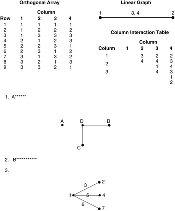
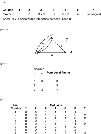
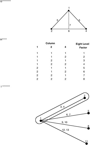
Figure 9.10: The orthogonal array (OA), linear graph (LG), and column interaction for L9.

INTERACTIONS AND HARDWARE TEST SETUP

The orthogonal array specifies the hardware setup for each test. To set up the hardware for a particular test in the orthogonal array, the experimenter should disregard the interaction columns and use only the columns assigned to single factors. If an interaction is included in the experiment, its level will be based solely upon the levels of the interacting factors. The interaction will come into consideration during the analysis of the data. An example will demonstrate the use of the linear graph and the layout of a simple experiment.

A brainstorming group has constructed a cause-and-effect diagram and determined that four factors (A through D) are suspected of being contributors to the problem. In addition, two interactions are suspected (B — D and C — D). The group has decided to use two levels for each factor. The experiment is laid out as follows:

1. Determine the df requirement.

   Four dfs are required for the main factors (one for each two level factor).

   Two dfs are required for the interactions (one for each interaction of two level factors).

   Six dfs are required in total.

2. Determine a likely orthogonal array.

   Since 6 dfs + 1 = 7 tests minimum and all factors have two levels, the L8 array is a likely place to start.

3. Draw the linear graph required for the experiment.

   The linear graph required for the experiment is shown in Figure 9.10A.

4. Compare the linear graph(s) of the orthogonal array to the linear graph required for the experiment.

   One of the linear graphs for the L8 that could fit is shown in Figure 9.10B.

5. Assign factors to the orthogonal array columns.

   Make the column assignments shown in Figure 9.10C.

 

CHOICE OF THE TEST ARRAY

For a particular experiment, the test response should be chosen to minimize interaction, and the smallest orthogonal array that fits the situation should be used. The emphasis should be on assigning factors to as many columns as possible. This allows the question posed by the situation to be answered using a minimum number of tests.

Whether an interaction exists or not is an important issue that must be addressed in setting up the experiment. If an interaction does exist and provision is not made for it in the experimental setup, its effect becomes "mixed up" or confounded with the effect of the factor assigned to the column where the interaction would be assigned. The analysis will not be able to separate the two. This is an important reason why confirmatory runs are necessary. Confirmatory runs should be made with the nonsignificant factors set to their different levels, just to make sure.

Another way to minimize the effect of interactions is to use an L12, L18, or L36 orthogonal array. These arrays have a special property that some, or all, of the interactions between columns are spread across all columns more or less equally instead of being concentrated in a column. This property can be used by the experimenter to rank the contribution of factors without worrying about interactions. There are times when this can be a valuable tool for the experimenter. The linear graphs for those arrays tell which interactions can be estimated and which cannot.

FACTORS WITH FOUR LEVELS

A factor with four levels can easily be assigned to a two-level orthogonal array. A four-level factor requires 3 dfs. Since a two-level column has 1 df, three two-level columns are used for the four-level factor. The three columns chosen must be represented in the linear graph by two dots and the connecting interaction line. One of the L8 linear graphs is shown in Figure 9.10D.

The line enclosing the column 1, 2, 3 designators indicates that these columns will be used for a four-level factor. The particular level of the four-level factor for each run can be determined by taking any two of the three columns that are to be combined and assigning the four combinations to the four levels of the factor. As an example, consider columns 1 and 2 (see Figure 9.10E).

Although column 3 is not used in determining the level of the four-level factor, its df is used and no other factor can be assigned to it.

In the orthogonal array, one of the columns used for the four-level factor is set to the levels of the four-level factor and the other two columns are set to zero for each test. For the L8 example, the modified array would be Figure 9.10F.

FACTORS WITH EIGHT LEVELS

In a similar manner, a factor with eight levels requires 7 dfs and takes up seven two-level columns. The particular columns are chosen by taking a closed triangle in the linear graph and the interactions column of one of the points of the triangle with the opposite base. One example is shown in Figure 9.10G.

The column interaction table indicates that the interaction of columns 1 and 6 will be in column 7. The actual factor level for each test is determined by looking at the combinations of the three columns that make up the corners of the triangle (see Figure 9.10H).

None of the seven columns which are used for the eight-level factor can be assigned to another factor. In the orthogonal array, one of the columns used for the eight-level factor is set to the levels of the eight-level factor and the other six columns are set to zero for each test.

FACTORS WITH NINE LEVELS

A factor with nine levels is handled in a similar manner to a four-level factor. The nine-level factor requires 8 dfs, which are available in four three-level columns. Two three-level columns and their two interaction columns are used. One of the L27 linear graphs is shown in Figure 9.10I.

The line enclosing the column 1, 2, 3, 4 designators indicates that these four columns will be used for the nine-level factor. The level of the nine-level factor to be used in a particular test can be determined by taking any two of the four columns that are to be combined and assigning their nine combinations to the nine levels of the factor. This is left to the reader to demonstrate.

In the orthogonal array, one of the columns used for the nine-level factor is set to the levels of the nine-level factor and the other three columns are set to zero.

USING FACTORS WITH TWO LEVELS IN A THREE-LEVEL ARRAY

Dummy Treatment

Often, the situation calls for a mix of factors with two and three levels. A two-level factor can be assigned to a three-level column by using one of the two levels as the third level in the test determination. Consider using a two-level factor in an L9 array ” see Table 9.11.

Table 9.11: An L9 with a Two-Level Column

Test Number	Columns
	1	2	3	4
1	1	1	1	1
2	1	2	2	2
3	1	3	3	3
4	2	1	2	3
5	2	2	3	1
6	2	3	1	2
7	1	1	3	2
8	1	2	1	3
9	1	3	2	1

In column 1, the second set of 1s (in experiments 7, 8, and 9) is the dummy treatment. In the analysis, the average at level one of the factor assigned to column 1 is determined with more accuracy than the average at level two since more tests are run at level one. The level that is of more interest to the experimenter should be the one used for the dummy treatment.

Combination Method

Two two-level factors can be assigned to a single three-level column. This is done by assigning three of the four combinations of the two two-level factors to the three-level factor and not testing the fourth combination. As an example, two two-level factors are assigned to a three-level column as in Table 9.12. Note that the combination A ₂ B ₂ is not tested. In this approach, information about the AB interaction is not available, and many ANOVA (analysis of variance) computer programs are not able to break apart the effect of A and B. A way of doing that manually will be presented later.

Table 9.12: Combination Method

Factor A	Factor B	Three-Level Column
1	1	1
1	2	2
2	1	3

USING FACTORS WITH THREE LEVELS IN A TWO-LEVEL ARRAY

A factor with three levels requires 2 dfs. Although it would seem that two two-level columns combined would give the required dfs, the interaction of those two columns is confounded with the three-level factor. The approach used to assign one three-level factor to a two-level array is to construct a four-level column and use the dummy treatment approach to assign the three-level factor to the four-level column.

Assigning more than one three-level factor to a two-level array uses a variation of this approach. Recall that in constructing a four-level column, three two-level columns are used. These three must be shown in the linear graph as two dots connected by an interaction line. Any two of these columns are used to determine the level to be tested. The third column's df is used up in assigning a four-level factor. In assigning a three-level factor, the third column's df is not used for the level three factor since it require only 2 dfs. However, the third column is confounded with the three-level factor and should not be assigned to another factor. That column is said to be "idle." When two or more three-level factors are assigned to a two-level array, the three-level factors can share the same idle column. An example of assigning two three-level factors to an L8 array is shown in Figure 9.11.

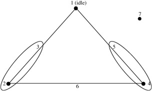
Figure 9.11: Three-level factors in a L8 array.

Here column 1 would be idle (a factor cannot be assigned to column 1), columns 2 and 3 would be used to determine the levels of a three-level factor, columns 4 and 5 would be used to determine the levels of the second three-level factor, and columns 6 and 7 are available for two-level factors. The modified orthogonal array for this experiment is shown in Table 9.13 (level 2 is the dummy treatment in both cases).

Table 9.13: Modified L8 Array

Test Number	Columns
	1	2	3	4	5	6	7
1	1		1		1	1	1
2	1		1		2	2	2
3	1		2		1	2	2
4	1		2		2	1	1
5	2		3		2	1	2
6	2		3		3	2	1
7	2		2		2	2	1
8	2		2		3	1	2

The idle column approach cannot be used with four-level factors. If it were attempted, insufficient degrees of freedom would exist and the four-level factors would be confounded.

OTHER TECHNIQUES

There are other techniques for setting up an experiment that will be mentioned here but will not be discussed in detail. The user is invited to read the chapter on pseudo-factor design in Quality Engineering ” Product and Process Design Optimization , by Yuin Wu and Dr. Willie Hobbs Moore or to consult with a statistician to use these techniques.

Nesting of Factors

Occasionally, levels of one factor have meaning only at a particular level of another factor. Consider the comparison of two types of machine. One is electrically operated and the other is hydraulically operated. The voltage and frequency of the electrical power source and the temperature and formulation of the hydraulic fluid are factors that have meaning for one type of machine but not the other. These factors are nested within the machine level and require a special setup and analysis which is discussed in the reference given above.

Setting Up Experiments with Factors with Large Numbers of Levels

Experiments with factors with large numbers of levels can be assigned to an experimental layout using combinations of the techniques that have been covered in this booklet.

INNER ARRAYS AND OUTER ARRAYS

Factors are generally divided into three basic types:

1. Control factors are the factors that are to be optimized to attain the experimental goal.

2. Noise factors represent the uncontrollable elements of the system. The optimum choice of control factor levels should be robust over the noise factor levels.

3. Signal factors represent different inputs into the system for which system response should be different. For example, if several micrometers were to be compared, the standard thickness to be measured would be levels of a signal factor. The optimum micrometer choice would be the one that operated best at all the standard thicknesses. Signal factors are discussed in more detail on pages 430 “441.

Control and noise factors are usually handled differently from one another in setting up an experiment. Control factors are entered into an orthogonal array called an inner array. The noise factors are entered into a separate array called an outer array. These arrays are related so that every test setup in the inner array is evaluated across every noise setup in the outer array. As an example, consider an L8 inner (control) array with an L4 outer (noise) array, as shown in Table 9.14.

Table 9.14: An L8 with an L4 Outer Array

Test No.	L8							L4 (on side) ’	1	2	2	1
									1	2	1	2
	1	2	3	4	5	6	7		1	1	2	2
1	1	1	1	1	1	1	1	Test Results	x1	x2	x3	x4
2	1	1	1	2	2	2	2		x5	x6	x7	x8
3	1	2	2	1	1	2	2
4	1	2	2	2	2	1	1		.	.	.	.
5	2	1	2	1	2	1	2		.	.	.	.
6	2	1	2	2	1	2	1		.	.	.	.
7	2	2	1	1	2	2	1
8	2	2	1	2	1	1	2		x29	x30	x31	x32
Note: The x values refer to experimental test results.

The purpose of this relationship is to equally and completely expose the control factor choices to the uncontrollable environment. This ensures that the optimum factor will be robust. A signal-to-noise (S/N) ratio can be calculated for each of the control factor array test situations. This allows the experimenter to identify the control factor level choices that meet the target response consistently.

RANDOMIZATION OF THE EXPERIMENTAL TESTS

In the orthogonal arrays, each test setup is identified by a test number. Generally, the tests should not be run in the order of test number. If the tests were run in that order, all the tests with the factor assigned to column one at level one would be run before any of the tests with that factor at level two. A quick glance at an orthogonal array will confirm this relationship. In fact, the columns toward the left of the array change less often than the columns toward the right of the array. If an uncontrolled noise factor changes during the testing process, the effect of that noise factor could be mixed in with one or more of the factor effects. This could result in an erroneous conclusion. The possibility of this occurring can be minimized by randomizing the order of the experiment runs. If the order of the tests is randomized, the effect of the changing uncontrolled noise factor will be more or less spread evenly over all the levels of the controlled factors and although the experimental error will be increased, the effects of the controlled factors will still be identifiable. Randomization can be done as simply as writing the test numbers on slips of paper and drawing them out of a hat.

There are two situations where randomization may not be possible or where its importance is lessened.

1. If it is very expensive, difficult, or time-consuming to change the level of a factor, all tests at one level of a factor may have to be run before the level of that factor can be changed. In this case, noise factors should be chosen for the outer array that represent the possible variation in uncontrolled environment as much as possible.

2. If the noise factors in the outer array are properly chosen, the confident experimenter may elect to dispense with randomization. In most cases, the purpose of the experiment is to learn more about the situation, and the experimenter does not have complete confidence. Therefore, the test order should be randomized whenever the circumstances permit.

MISCELLANEOUS THOUGHTS

Dr. Taguchi stresses evaluating as many main factors as possible and filling up the available columns. If it turns out that the experimental design will result in unassigned columns, some column assignment schemes are better than others in a few situations. The rationale behind these choices is that they minimize the confounding of unsuspected two-factor interactions with the main factors. A detailed discussion is beyond the scope of this chapter. The user is invited to read Chapter 12 of Statistics for Experiments , by G. Box, W. Hunter, and J.S. Hunter to learn more about this concept.

Consider an L8 for which there are to be four two-level factors assigned. This implies that there will be three columns that will not be assigned to a main factor. There are 35 ways in which the four factors can be assigned to the seven columns. The recommended assignment is to use columns 1, 2, 4, and 7 for the main factors. The interactions to be evaluated, the linear graphs, and the column interaction table determine if the recommended column assignments are usable for a particular experiment. The recommended column assignments are given in Table 9.15.

Table 9.15: Recommended Factor Assignment by Column

Number of Factors	L8 Array	L16 Array	L32 Array
4	1, 2, 4, 7	1, 2, 4, 8
5	[a]	1, 2, 4, 8, 15	1, 2, 4, 8, 16
6	[a]	1, 2, 4, 8, 11, 13	1, 2, 4, 8, 16, 31
7	[a]	1, 2, 4, 7, 8, 11, 13	1, 2, 4, 8, 15, 16, 23
8	”	1, 2, 4, 7, 8, 11, 13, 14	1, 2, 4, 8, 15, 16, 23, 27
9	”	[a]	1, 2, 4, 8, 15, 16, 23, 27, 29
10	”	[a]	1, 2, 4, 8, 15, 16, 23, 27, 29, 30
11	”	[a]	1, 2, 4, 7, 8, 11, 13, 14, 16, 19, 21
12	”	[a]	1, 2, 4, 7, 8, 11, 13, 14, 16, 19, 21, 22
13	__	[a]	1, 2, 4, 7, 8, 11, 13, 14, 16, 19, 21, 22, 25
14	__	[a]	1, 2, 4, 7, 8, 11, 13, 14, 16, 19, 21, 22, 25, 26
15	”	[a]	1, 2, 4, 7, 8, 11, 13, 14, 16, 19, 21, 22, 25, 26, 28
[a] No recommended assignment scheme.

Some of the linear graphs may be found in the Appendix of Volume V. However, the user will find that the linear graphs in other books and reference materials may not make these assignments available. There are many equally valid ways that linear graphs for the larger arrays can be constructed from the column interaction table. It is not feasible for any one book to list all the possibilities. An excellent source is Taguchi and Konishi (1987).

In many cases, the brainstorming group may not have a good feel for whether interactions exist or not. In these cases, two alternatives are usually considered:

1. Design an experiment that allows all two-factor interactions to be estimated.

2. Design an experiment in which no factor is assigned to a column that also contains the interaction of two other factors, although pairs of two-factor interactions may be assigned to the same column. The recommended factor assignments given in Table 9.15 are examples of this approach.

The second approach is based on the assumption that few of the interactions will be significant and that later testing can be used to investigate them in more detail. The reader is urged to seek statistical assistance in approaching this type of experiment.

Sometimes, the response is not related to the input factors in a linear fashion. Testing each factor at two levels allows only a linear relationship to be defined and, in this more complex situation, can give misleading results. A detailed statistical analysis tool called response surface methodology can be used to investigate the complex relationship of the input factors to the response in these cases.

All of this seems to indicate that DOEs must be lengthy and complicated when interactions or nonlinear relationships are suspected. In most situations, time and resources are not available to run a large experiment. Sometimes, a transformation of the measured data or of a quantitative input factor can allow a linear model to fit within the region covered by the input factors. The linear model requires fewer data points than a curvilinear model and is easier to interpret. Unfortunately, unless multiple observations are made at each inner array setup, the choice of transformation is guided mainly by the experience of the experimenter or by trying several transformations and seeing which one fits best.

The choice of the proper transformation to use is related to the choice of the proper response. As an example, two common measures of fuel usage are "miles per gallon" and "liters per kilometer." With the multiplication of a constant, these two measures are inverses of each other. A model that is linear in mi/g will be definitely non-linear in 1/km. Which measurement is correct? There is no easy answer. The experimenter should evaluate several different transformations to determine the best model. Some transformations that are useful are:

y	=	Y 1/2 useful for count data (Poisson distributed) such as the number of flaws in a painted surface
y	=	log(Y) or ln(Y)useful for comparing variances
y	=	Y -1/2
y	=	1/Y

When there are several observations at each inner array test setup either through replication or through testing with and outer array, another guide to choosing the right transformation can be used. For the ANOVA to work correctly, the variances at all test points should be equal. The observed variances should be compared as follows:

1. Calculate the average and the standard deviation(s) for each inner array test setup.

2. Take the log or ln of each and s.

3. Plot log s (y-axis) versus log (x-axis) and estimate the slope.

4. Use the estimated slope as a rough guide to determine which transformation to use:

   Slope	Transformation
   0.0	no transformation
   0.5	y = Y 1/2
   1.0	y = log(Y) or ln(Y)
   1.5	y = Y -1/2
   2.0	y = 1/Y

It should be noted that the addition or subtraction of a constant before plotting will not affect the standard deviation but will affect the relative spacing of the log and hence the slope of the line. This approach can be used to improve the fit of the transformation. With the widespread use of computers, data analysis of this type should be easy and should be pursued as a means to get the most information out of the data.

Examples of this approach will be given later in the chapter. The reader is invited to refer to Statistics for Experiments by G. Box, W. Hunter, and J.S. Hunter to learn more about the use of transformations in analyzing data.