Understanding Performance Bottlenecks

EXAM 70-293 OBJECTIVE 4, 4.1, 4.2

All system administrators want the systems they install to run perfectly out of the box, all the time. We have all wanted to be able to safely turn off our pagers and cell phones. Our servers should run reliably, quickly, and without interruption, right? Well, if that were the case, we would all be terminally bored or changing careers.

In this chapter, we will examine the conditions and tools for monitoring and ensuring a system’s smooth operation. In Chapter 9, we will discuss some of the sophisticated tools Microsoft has included with Windows Server 2003 for enhancing system uptime and supporting high-volume use.

Identifying System Bottlenecks

For the most part, a Windows Server 2003 system does run well in its default configuration, and, if designed and maintained properly, operates with a minimum of administrative overhead. However, as a general-purpose operating system, it can often be tuned to perform better when used for certain tasks.

The main hardware resources of any computer system are memory, processor, disk storage, and communications or network components. Different applications and circumstances use these resources in different combinations, often taxing one resource more than another. If multiple applications are run on a system, it is often possible to reach the limit of a resource and suffer slow response time, unreliable services, or miss a result. We will take a look at each of these resources, discuss some of the common issues related to them, and consider some of the management options available.

Memory

Memory, random access memory, or simply RAM is the working space of the operating system and applications. Its contents are volatile and always in demand. In 1990, a computer system that had a memory capacity of 16MB was very high end. Today, it is possible to purchase systems that support 32GB of memory or more.

RAM is most often the single resource that becomes a bottleneck. A common cause of slow performance is insufficient physical memory. When purchasing new hardware, it is not wise to skimp on memory. The minimum recommended amount of memory for running Windows Server 2003 is 128MB (512MB for Datacenter Edition). These are very conservative numbers. Even Microsoft recommends at least 256MB. If you have the ability, double (or more) the amounts to, and you will be happy you did. The short rule with memory is this: more is better.

The Windows operating system controls the access to and allocation of memory and performs “housekeeping tasks” when needed. Applications request memory from the operating system, which allocates memory to the application. When an application no longer needs memory, the application is supposed to release the memory back to the operating system. An application that does not properly release memory can slowly drain a system of available free memory, and overall performance will suffer. This is referred to as a memory leak.

Another performance factor related to memory is the use of virtual memory (VM) or paging. Virtual memory is a method of increasing the amount of memory in a system by using a file on the hard drive called a page file. The apparent size of memory is increased without increasing the physical RAM in the system, hence the term virtual. Access to hard drives, even on the fastest disk subsystems, is dozens or hundreds of times slower than access to RAM. When the operating system needs more RAM than is available, it copies the least recently used pages of memory to the page file, and then reassigns those pages of RAM to the application that requested it. The next time a memory request occurs, the operating system may need to reallocate more pages in RAM or retrieve pages from the page file. This paging process can slow even the fastest system.

Tuning memory is often as simple as adding more memory, reducing the number of applications running (including applications that run in the System Tray), or stopping unnecessary services. However, there is an advanced memory-tuning technique that can be applied if the application supports it. Part of the Enterprise Memory Architecture feature of the Enterprise and Datacenter editions of Windows Server 2003 is 4GB tuning (4GT), also called application memory tuning. Using this feature, you can change the amount of RAM addressable by applications from 2GB to 4GB. Your system must have at least 2GB of physical RAM installed, and the application must be written to support the increased memory range. Consult the application documentation or contact your vendor to make this determination.

Head of the Class...
Page File Tricks

Configuring the Windows page file is not as simple as it may seem. Several factors can affect the performance of the page file and therefore overall system performance. The page file is heavily accessed. Placing it on separate drive and control channel from the operating system and/or applications greatly reduces competition for disk access (known as contention).

Spreading the page file across several drives and control channels can boost performance as well, provided that the pieces are not stored on high-contention drives. The use of high-performance drives will also improve performance. In general, SCSI and Fibre Channel provide greater performance than IDE drives.

Keeping the page file defragmented will also help its performance. A single contiguous block of disk space provides better performance by reducing drive read/write head movement. Before adding a new page file to a drive, use the Windows Disk Defragmenter utility to defragment the disk. When you add the new page file to the disk, it will automatically allocate as much contiguous space as it can.

Finally, consider using the Custom Size option when configuring virtual memory, and make the Initial Size and Maximum Size options the same value. This will consume more disk space but will avoid any incidents of expansion delay, which occurs when the system must increase the size of the page file. This will also help keep the page file defragmented.

Finally, remember that even the most optimally tuned page file configuration will not make up for insufficient physical RAM.

Processor

If memory is the working space, then the processor is the worker. The central processing unit, or CPU, is the “brain” of a computer system and is responsible for, well, processing. It receives data (input), performs calculations (execution), and reports the result (output). The processor is (usually, but not always) responsible for moving data around inside a computer system, transporting it among memory, disk, network, and other devices.

CPUs are commonly described by their type, brand, or model (for example, Pentium 4), and their clock speed (for example, 2.0 GHz). In simplest terms, the clock speed is how many times per second the CPU executes an instruction. Generally, the faster the CPU is, the better the computer performs.

The CPU bus architecture is another factor when examining performance. Bus architecture is a term used to describe how much data can be moved in and out of the processor at once. It also describes the amount of information that the CPU can process in a single step. A 32-bit CPU (which includes all of Intel’s CPUs from the 80386 through the Pentium 4 and AMD’s CPUs from the Am486 through the Athlon-XP) can use 32 bits wide and access 232 bytes of memory, or 4GB. A 64-bit CPU (Intel’s Itanium series and AMD’s Opteron series) can use 64 bits wide and access (in theory) 264 bytes of memory or 16 exabytes (16 billion gigabytes). No current hardware can support this amount of RAM. Windows Server 2003 supports a maximum of 512GB on Itanium-based hardware with the Datacenter Edition. The point is that 64-bit CPUs can support significantly more memory and run applications that use more of it than 32-bit CPUs, all at a faster speed. Extremely large databases can get a large performance boost on 64-bit systems.

Using multiple CPUs in a computer (called multiprocessing) allows a computer system to run more applications at the same time than a single-CPU system, because the workload can be spread among the processors. In effect, this reduces the competition among applications for CPU time. A related programming technology called multithreading allows the operating system to run different parts of an application (threads) on multiple CPUs at the same time, spreading out the workload. Windows Server 2003 can support up to 64 CPUs, depending on the edition of the operating system in use.

A recent development by Intel is a technology called hyperthreading. This feature, introduced in the Xeon and Pentium 4 series of processors, makes a single CPU appear to be two CPUs. Hyperthreading is implemented at the BIOS level and is therefore transparent to the operating system. It typically yields a performance increase of 20 to 30 percent, meaning it is not as efficient as multiple physical CPUs. However, it is included for free on hardware that supports the technology.

One of the downsides of multiple processors is the management of interrupts. An interrupt is a hardware or software signal that stops the current flow of instructions in order to handle another event occurring in the system. Disk input/output (I/O), network I/O, keyboard activity, and mouse activity are driven by interrupts. Interrupts are a necessary part of the computer’s operation, but they can impact the performance of a multiprocessor system. The first CPU in a multiprocessor system (processor 0) controls I/O. If an application running on another CPU requires a lot of I/O, CPU 0 can spend much of its time managing interrupts instead of running an application. Windows Server 2003 manages multiple processors and interrupts quite well, but there is a way to tune the affinity of a thread to a specific processor.

Processor affinity is a method of associating an application with a specific CPU. Processor affinity can be used to reduce some of the overhead associated with multiple CPUs and is controlled primarily via the Task Manager utility.

Priority is a mechanism used to prioritize some applications (or threads) over others. Priority can be set when an application is started or can be changed later using the Task Manager utility.

Disk

The disk (interchangeably called hard disk, drive, storage, permanent storage, array, spindles, or multiple combinations of these terms) is the permanent storage location of the operating system, applications, and data. A disk is made up of one or more physical drives. Disk content remains when power is turned off. Often, a computer system will contain multiple disks configured in arrays, which can be useful for increasing performance and/or availability.

Several factors contribute to the performance and reliability of disk:

• The disk controller technology

• The life-expectancy or mean time of the drive(s)

• The way data is arranged on the drive(s)

• The way data is accessed on the drive(s)

• The ratio of drive controllers to the number of drives

Disk Controller Technology

The hard drive itself is a dependent component, meaning it requires some other device to interface with the computer system. The component that provides this interface is the disk controller. The disk controller is responsible for converting the request of the operating system into instructions the hard drive can process. The controller also manages the flow of data to and from the drive. A hard drive is always manufactured to work with a specific type of controller.

There are three major types of hard drive interface technologies, each with their own advantages and disadvantages. ATA (sometimes called IDE or EIDE) is the most common interface. Though often found on server-class systems, its primary usage is on workstation-class or midrange systems. Compared to the other technologies, ATA drives usually cost the least. The ATA interface itself can support a maximum achievable throughput of about 50 Megabytes per second (MBps). ATA systems generally support four drives, with two drives on a disk channel. One drive on the channel is configured as master, and the other (if present) is configured as slave. This configuration means that the master drive controls the traffic on the channel as well as the slave drive. This can raise some hardware incompatibility issues, and it is for this reason that you should not mix drives from different manufacturers on the same channel if you can avoid doing so. ATA was designed primarily for use with disk drives, but other ATA devices do exist, such as CD/DVD-ROM drives and tape drives.

The second interface technology commonly used is the Small Computers System Interface, commonly called SCSI (pronounced “skuzzy”). As a defined technology, SCSI has been around longer than ATA, but it is less prevalent because SCSI devices are generally more expensive than similar ATA devices. SCSI is most commonly found on midrange to high-end server systems. SCSI is a general-purpose interface technology that supports a wide variety of devices: hard drives, tape drives, CD and DVD-ROM drives, scanners, write once/read many (WORM) drives, and more. A SCSI channel can support from 8 to 16 devices, depending on the exact SCSI specification being followed. The current SCSI specification supports 16 devices and a bus speed of 160 MBps. The SCSI bus controller is considered intelligent, meaning that the controller, rather than the system CPU (as is the case with ATA), does the work of managing the channel and the flow of data on the channel. This gives SCSI a performance advantage over ATA but requires SCSI devices to have more advanced circuitry, increasing the cost of SCSI devices.

Fibre Channel (sometimes referred to as F/C) is the most recent interface technology to come into widespread use. It is not usually built into a system and requires interface adapters to be installed. Fibre Channel is commonly used to connect servers to large back-end storage area networks (SANs). Data rates of 100 MBps, 1000 MBps, and 2000 MBps are possible with Fibre Channel. Fibre Channel is quite expensive, but it supports hundreds of devices per channel. When connected via an SAN, a Fibre Channel configuration can supports thousands of devices. Because Fibre Channel can support such a large number of devices, a Fibre Channel configuration can be very complex and difficult to manage. Like SCSI, Fibre Channel is a general-purpose interface technology and supports many devices other than disk drives. Because of its higher cost, however, there are generally fewer devices available for Fibre Channel than for SCSI.

Drive Life Expectancy (MTBF)

Because hard drives contain rapidly rotating moving parts, they are subject to more frequent mechanical failure than most other components in a computer system. Disk drive manufacturers usually predict the rate of failure in terms of mean time between failures (MTBF). This number is often measured in thousands of hours of operation and is an indicator of the statistical reliability of the hard drive device.

It is quite possible to see MTBF ratings of 100,000 hours (11.4 years) or more. But what happens with multiple drives? By understanding that drive failure is a real and predictable event, you can calculate the likelihood of your system experiencing a drive failure. For example, if you were to install two identical hard drives in your system, each with a MTBF of 100,000 hours, when would you (statistically) expect to experience a drive failure? The answer is sometime within 5.7 years (100,000 MTBF hours/2 drives). This may not seem like too much of an issue until you extend the calculation. It is not uncommon for systems to have six or more drives, depending on the amount of storage needed and the size of the drives involved. Using the same 100,000-hour example with six drives, you could expect to see a failure sometime within 23 months, or just less than two years. If you have more disks, the odds turn against you even further. In short, the more drives you have, the higher the likelihood of experiencing a drive failure.

The mechanism used to control the cumulative effect of this problem is Redundant Arrays of Independent Disks, or RAID. RAID is a technique of using multiple drives in such a way that data is spread among the drives so that, in the event of failure, the data is available from either a second copy of the data or is re-creatable from a mathematical calculation. A properly configured RAID array counteracts the cumulative effect of MTBF.

RAID arrays can also be used to increase performance. For example, if you were using five disk drives and spread the data evenly among those drives, you would expect to see it take one-fifth the time to read the data from that array than from a single drive containing the same data. This is referred to as increasing the spindle count. (The spindle is the axle that the disks in the disk drive are attached to.) By increasing the number of spindles, you reduce the demand on any single drive for reads or writes.

RAID is configured in one of two ways: in software or in hardware. Software RAID is supported by Windows Server 2003 and can be used to create and manage some types of RAID arrays without the cost of a hardware RAID controller. Hardware RAID requires a hardware RAID controller and usually offers more options for configuring a RAID array, as well as increased performance over software RAID.

Arrangement of Data on Drives

How data is arranged on a drive affects how fast the data is written to a drive or read from a drive. Assume that you are starting with a clean, freshly formatted hard drive. As files are written to the drive, they are assigned to available areas of the disk (called clusters) by the file system. If the file is large enough, it will be written to multiple clusters. If a file occupies clusters that are next to each other on disk, the file is said to occupy contiguous clusters. Over time, additional files are written to the disk. Later, your first file increases in size. The file system allocates new clusters to the file, some of which it already occupied and some of which are now on a different area of the disk. The file no longer occupies contiguous clusters and is fragmented; multiple fragments of the file are spread out around the disk. The effect of fragmentation is to require more time to access the file, thus slowing performance. Fragmentation occurs on every drive, but frequently updated drives are most susceptible to the performance degradation of fragmentation.

Microsoft recognizes that file fragmentation can be a problem and has included a utility with Windows Server 2003 to address this problem. You can use the Disk Defragmenter utility to reduce the total fragmentation on a drive. This utility can be started from the command line or from the Start menu, as shown in Figure 8.1.

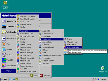
Figure 8.1: Starting Disk Defragmenter

Although file fragmentation can have an impact on performance, so can the cure. While running, Disk Defragmenter can have a serious performance impact on a system. It is for this reason that you should use Disk Defragmenter with caution. You can use the Analysis function of Disk Defragmenter to see the fragmentation statistics on a drive without actually performing defragmentation.

New & Noteworthy...
Scheduling Disk Defragmenter

One of the great features missing in Windows NT 4 and limited in Windows 2000 is the Disk Defragmenter utility. It was originally thought that because of the way NTFS functions, file fragmentation would not be an issue. This thinking was proven wrong, however, in the earliest versions of Windows NT, and an appropriate application program interface (API) was built into Windows NT 4 to support defragmentation. Although Microsoft did not include a defragmentation tool in the operating system, a few third-party software publishers produced successful defragmentation products for that operating system.

In Windows 2000, Microsoft included the first version of the Disk Defragmenter utility. This version performed defragmentation adequately, but could run only interactively. This meant that defragmentation needed to be performed by an administrator sitting at the console or via a Terminal Services session. Well, Microsoft has made a nice improvement.

Disk Defragmenter in Windows Server 2003 can be run from the Start menu or from the command line (Defrag.exe). Although Disk Defragmenter has no built-in scheduling function, if you run it from the command line, you can use the AT job-scheduling command to create a scheduled defragmentation run. You no longer need to be logged in to the server to run a defragmentation procedure.

If you’ve ever needed to manually defragment a lot of servers, you’ll appreciate this new capability. If you’ve never performed a lot of manual defragmentation runs, consider yourself very fortunate to have this feature available now.

The Way Data Is Accessed on Drives

Different applications access data in different ways. For example, Microsoft Exchange Server will write to transaction logs sequentially; the mail store databases may be written to and read from either randomly or sequentially. You should be able to develop a profile of this pattern of reads and writes. This profile will determine the design of the underlying disk system and RAID type used. If the wrong RAID type is used, performance will suffer and/or reliability will be compromised.

If you are running multiple I/O-intensive applications on a system, consider giving each application its own drives and controller. That way, the applications will not conflict with each other for I/O resources.

The Ratio of Drive Controllers to the Number of Drives

The ratio of drive controllers to the number of drives relates to the way data is accessed on drives. As mentioned earlier, a higher number of spindles can yield higher throughput. However, if all the drives are connected to one controller, the controller can potentially become a bottleneck, because all I/O must go through the controller. In systems with multiple drives, it may be beneficial to add more controllers and balance the drives among the controllers. This reduces the load on any one controller and results in improved throughput.

Another potential performance improvement with multiple controllers is the ability of the operating system to perform split seeks. If the drives on the controllers are mirrored, the operating system will send read requests to the drive that is able to service the request the quickest.

Network Components

A network is the primary computer-to-computer communications mechanism used in modern computing environments. Windows Server 2003 supports numerous network interface cards (NICs) and multiple network topologies, including Ethernet, Token Ring, Asynchronous Transfer Mode (ATM), and Fiber Data Distributed Interconnect (FDDI), as well as remote-access technologies including dial-up and virtual private Network (VPN) connections.

The primary (and default) communications protocol used by Windows Server 2003 is TCP/IP. The operating system also supports the next generation of the TCP/IP protocol, IP version 6 (IPv6), as well as the AppleTalk, Reliable Multicast, and NWLink protocols. Multiple protocols installed on a system consume additional memory and CPU resources. Reducing the number of protocols in use will improve performance.

On systems that do have multiple protocols loaded, change the binding order of the protocols to the NIC so that the most frequently used protocol is bound first. This will reduce the amount of processing needed for each network packet and improve performance.

When a packet is received by the NIC, it is placed in a memory buffer. The NIC then either generates an interrupt to have the CPU transfer the packet to the main memory of the computer or performs a direct memory access (DMA) transfer and moves the data itself. The method used depends on the hardware involved. The DMA transfer method is much faster and has less impact on the overall system.

The number and/or size of the memory buffers allocated to the NIC can affect performance as well. Some NICs allow you to adjust the number of memory buffers assigned to the card. A larger buffer space allows the NIC to store more packets, reducing the number of interrupts the card must generate by allowing larger, less frequent data transfers. Conversely, reducing the number of buffers can increase the amount of interrupts generated by the NIC, impacting system performance. Some NICs allow you to adjust the buffers for transmitting and receiving packets independently, giving you more flexibility in your configuration. The trade-off of increasing communication buffers may be a reduction in the amount of memory available to applications in the system.

One feature of Windows 2000 and Windows Server 2003 is support for IP Security (IPSec). This feature allows the securing of data transmitted over IP networks through the use of cryptography. IPSec is computer-intensive, meaning that significant amounts of CPU overhead are incurred with its use. Some NICs made in recent years support the offloading of the IPSec calculations to a highly optimized processor on the NIC. This can greatly reduce the amount of CPU time needed, as well as improve communications performance. NICs that support the offloading of IPSec are not much more expensive than regular NICs and should be strongly considered if you are using IPSec.

Another consideration for network performance is the network topology. Although it is not specific to the Windows operating system, network topology can greatly affect communications performance. If the traffic to your server must travel through routers that convert large incoming packets into multiple smaller packets, your server must do more work to reassemble the original packets before your applications can use the data. For example, if a client system is connected to a Token Ring network (which commonly uses a packet size of 4192 bytes or larger) and your server is connected via Ethernet (with a packet size of 1514 bytes), an intermediary router will “chop” the original packet into three or more packets for transmission on the Ethernet network segment. Your server must then reassemble these packets before passing them to applications. Reducing the number of topologies and/or routers on your network can improve performance by reducing packet conversions and reassembly.

Also, when using Ethernet, consider using switches instead of hubs. Switches are more expensive but allow higher communication rates and also permit more than one device to communicate at the same time. Hubs are cheaper but allow only one computer to be communicating at any given time. Switches are also not susceptible to Ethernet collisions, whereas hubs are at the mercy of collisions.

Another topology-related configuration is the duplex setting of the NICs. Primarily an issue with Ethernet, duplex describes how data is transmitted. A full-duplex communication link allows the simultaneous transmission and reception of data. Full duplex is the desired setting for servers, because servers normally need to transmit and receive at the same time. Full duplex typically requires switches. Half-duplex communication is the bi-directional communication of data but not at the same time. When transmitting data, receiving data is not possible and vice versa. Half duplex is often acceptable for workstations but should be avoided on servers.

Using the System Monitor Tool to Monitor Servers

EXAM 70-293 OBJECTIVE 4.2.1

Windows Server 2003 includes tools for monitoring the performance of your server. System Monitor is one such tool. System Monitor is an ActiveX control snap-in that is available as part of the Performance administrative tool. You can start it from the Start menu, as shown in Figure 8.2.

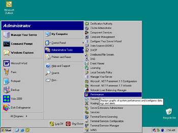
Figure 8.2: Starting the Performance Administrative Tool

System Monitor works by collecting information from counters built in to the operating system. Counters are features of the operating system (as well as some utilities and applications) that count specific events occurring in the system (like the number of disk writes each second or the percentage of disk space in use by files). The graphical view, shown in Figure 8.3, graphs the counter statistics.

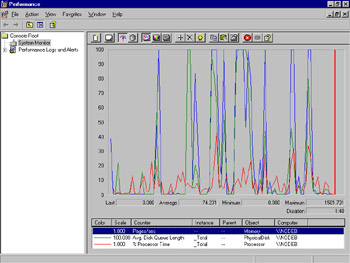
Figure 8.3: System Monitor, Graphical View with Default Counters

You can also see the counter statistics in System Monitor’s report view, as shown in Figure 8.4.

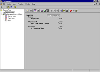
Figure 8.4: System Monitor, Report View with Default Counters

You can access the data collected by counters via System Monitor, other utilities, or third-party applications. This data provides you with an understanding of what is occurring on your system at the moment or over time. Using this information, you can tune your system’s operation to best suit your needs, determine if components are being overutilized, plan for expanding or replacing your system, or perform troubleshooting. Some of the most frequently used counters are shown in Table 8.1.

Table 8.1: Commonly Referenced Performance Counters

Resource	Performance Object:Counter	Recommended Threshold	Comments
Disk	Logical Disk: % Free Space	15%	Percentage of unused disk space. This value may be reduced on larger disks, depending on your preferences.
	Physical Disk: % Disk Time Logical Disk: % Disk Time	90%	If you’re using a hardware controller, try increasing the controller cache size to improve read/write performance. The Physical Disk counter is not always available or may be unreliable on clustered disks.
	Physical Disk: Disk Reads/sec Physical Disk: Disk Writes/sec	Varies by disk technology	The rate of read or write operations per second. Ultra SCSI should handle 50 to 70. I/O type (random/sequential) and RAID structure will affect this greatly.
	Physical Disk: Avg. Disk Queue Length	Total # of Varies spindles plus 2	The number of disk requests waiting to occur. It is used to determine if your disk system can keep up with I/O requests.
Memory	Memory: Available Bytes	Varies	The amount of free physical RAM available for allocation to a process or the system.
	Memory: Pages/sec	Varies	Number of pages read from or written to disk per second. Includes cache requests and swapped executable code requests.
Paging File	Paging File: % Usage	Greater than 70%	The percentage of the page file currently in use. This counter and the two Memory counters are linked. Low Available Bytes and high Pages/sec indicate a need for more physical memory.
Processor	Processor: % Processor Time	85%	Indicates what percentage of time the processor was not idle. If high, determine if a single process is consuming the CPU. Consider upgrading the CPU speed or adding processors.
	Processor: Interrupts/sec	Start at 1000 on single CPU; 5000 multiple	Indicates the number of hardware inter- rupts generated by the components of the system (network cards, disk controllers, CPUs and so on) per second. A sudden increase can indicate conflicts in hardware. Multiprocessor systems normally experience higher interrupt rates.
Server Work Queues	Server Work Queues: Queue Length	4	Indicates the number of requests waiting for service by the processor. A number higher than the threshold may indicate a processor bottleneck. Observe this value over time.
System	System: Processor Queue Length	Less than 10 per processor	The number of process threads awaiting execution. This counter is mainly relevant on multiprocessor systems. A high value may indicate a processor bottleneck. Observe this value over time.

Before you attempt to troubleshoot performance issues, you should perform a process called baselining. Baselining is the process of determining what the normal operating parameters are for your system. You develop a baseline by collecting data on your system in its initial state and at regular intervals over time. Save this collected data and store it in a database. You can then compare this historical data to current performance statistics to determine if your system’s behavior is changing slowly over time. Momentary spikes on the charts are normal, and you should not be overly concerned about them. Sustained highs can also be normal, depending on the activity occurring in a system, or they can signal a problem. Proper baselining will allow you to know when a sustained high is detrimental.

The Heisenberg Principal of physics (greatly paraphrased) states that you cannot observe the activity of something without altering its behavior. The same is true with performance monitoring. The collection of statistics requires computer resources. Collect only the counters you specifically need. If the system you wish to examine is extremely busy, consider using the noninteractive Performance Logs and Alerts function, shown in Figure 8.5, rather than System Monitor. Collecting the counters will still incur overhead, but not as much.

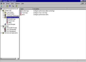
Figure 8.5: Performance Logs and Alerts, Accessed from Computer Management

You might also consider lowering the update interval or collecting data from the system on an hourly or daily basis, rather than continuously. If you’re monitoring disk counters, store the logs on a different disk (and, if possible, on a different controller channel) than the one you are monitoring. This will help avoid skewing the data. You can also save the collected statistics into a file or database, and then load and review them later (configured on the Source tab of the System Monitors Properties dialog box, shown later in Figure 8.12).

A counter log called System Overview, shown in Figure 8.6, is provided by Microsoft as an example. This log is configured to collect the same default counters as System Monitor at 15-second intervals.

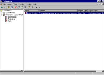
Figure 8.6: The Sample System Overview Counter Log

You can view the properties of the System Overview log by right-clicking it and selecting Properties from the context menu. Figure 8.7 shows the dialog box that appears.

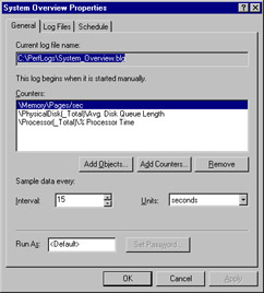
Figure 8.7: Properties of the System Overview Sample Log

The Log Files tab, shown in Figure 8.8, specifies the type (format) of the log file, its location, and the comment assigned to the log. The drop-down menu for the Log File Type option (shown in Figure 8.8) lists the formats available for log files. The binary format is compact and efficient. The text formats require more space to store the log, but they can be read by other applications like Microsoft Word and Excel. The binary circular file format overwrites itself when it reaches its maximum size, potentially saving disk space.

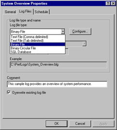
Figure 8.8: Properties of the System Overview Sample Log, Log Files Tab

If you click Configure… in the Log Files tab of the System Overview Properties dialog box, you will be presented with the Configure Log Files dialog box, as shown in Figure 8.9. Here, you can specify the location, name, and size limit of the log file.

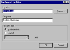
Figure 8.9: Configuring Log Files

The Schedule tab, shown in Figure 8.10, lets you specify the schedule for collecting data from the selected counters. The log can be manually controlled or can be scheduled to start at a specific date and time. You can stop the log manually or after a specific duration, a certain date and time, or when the log reaches its maximum size.

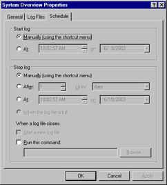
Figure 8.10: Properties of the System Overview Sample Log, Schedule Tab

By default, System Monitor tracks real-time data, but you can also have it display data from log files. To view log file data, click the View Log Data button in the main System Monitor window, as shown in Figure 8.11 (the icon that looks like a disk, the fourth from the left; circled for clarity in the figure).

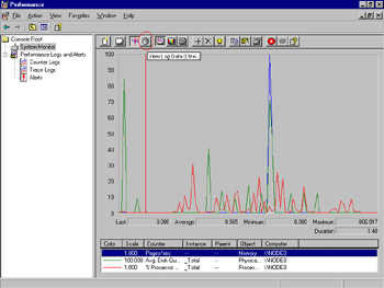
Figure 8.11: Selecting the View Log Data Button

On the Source tab, select the Log files option button and click Add. Browse to the log file you wish to view, select it, and click Open. With a log file added, the Source tab should look similar to Figure 8.12.

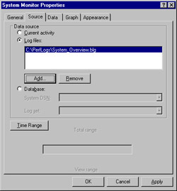
Figure 8.12: System Monitor Properties, Source Tab

Click OK, and you will be viewing the data collected in the log file. Figure 8.13 shows an example of viewing log file data.

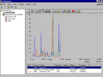
Figure 8.13: System Monitor, Viewing Log File Data

Determining if performance is acceptable can be highly subjective. It varies depending on the system, role, and environment. There are several general counters and specific thresholds for these counters that you can use to monitor performance. You should examine these counters as ratios over a period of regular intervals, rather than as the average of specific instances. This will provide a more realistic picture of the actual activity occurring on your system. In addition, watch for consistent occurrences of the threshold values being exceeded. It is not uncommon for momentary activity in a system to cause one or more counters to exceed threshold values, which may or may not be acceptable in your environment.

You can use System Monitor and Performance Logs and Alerts to monitor the local system or another computer on the network, as shown in Figure 8.14. It can be useful to compare the performance of the same resource on multiple systems. Be cautious when you do this, though. Ensure that you are comparing appropriately similar objects. Watch out for the “apples and oranges” mismatch. Also, consider that a server being monitored locally may have less monitoring overhead than one that is monitored remotely. This is particularly true regarding the network- and server-related counters, which can be skewed by the transmission of the performance data to your monitoring system. Be sure to account for this difference when developing your statistics.

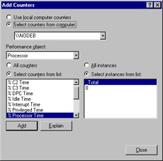
Figure 8.14: Selecting Counters from Another Computer

Note

You can also use System Monitor to track statistics from several different computers in the same log file or System Monitor graph. It can be very helpful to have all critical server data in one window or log, so that you can instantly spot problems on one or more of your servers by looking at a single screen.

If the Explain button in the Add Counters dialog box is not grayed out, a supporting explanation of the counter is available. The explanation for the Memory:Pages/sec counter is shown in Figure 8.15.

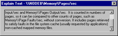
Figure 8.15: Viewing a Counter Explanation

Once you have become comfortable and proficient with reading counters, developing baselines, unobtrusively monitoring system activity, and comparing performance, you are ready for the final performance task: determining when your system will no longer be capable of performing the tasks that you want it to perform. Eventually, every computer will be outdated or outgrown. If you have developed the skills for monitoring your system, you should be able to determine in advance when your system will be outgrown. This will allow you to plan for the eventual expansion, enhancement, or replacement of the system. By taking this proactive approach, you can further reduce unplanned downtime by being prepared.

Note

Often overlooked, Task Manager is a useful tool for managing the system. Task Manager can assist you in getting an immediate picture of the activities occurring on your system. Stalled applications can be identified on the Applications tab. The amount of CPU and memory in use by each active process in the system is available on the Processes tab. The Performance tab provides a wealth of information on overall system activity, including a real-time bar graph for each processor in the system, showing the amount of time each is in use. The new Networking tab shows a real-time graph of the percentage of network bandwidth the system is using.

Exercise 8.01 will help you to become proficient in using System Monitor in the Performance console. You can complete the exercise from any Windows Server 2003 computer. Refer to Table 8.1, earlier in the chapter, for information about common counters.

Exercise 8.01: Creating a System Monitor Console

1. Select Start | All Programs | Administrative Tools | Performance. Click System Monitor. If any counters are already present, click the Delete (X) button on the toolbar, circled in Figure 8.16, until the System Monitor window is empty.

   
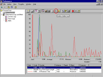
   Figure 8.16: Empty System Monitor

2. Click the Add (+) button on the toolbar. The Add Counters dialog box appears, as shown in Figure 8.17.

   
   Figure 8.17: Add Counters

3. In the Performance object drop-down list, select the Logical Disk object.

4. In the Select counters from list box, select the %Free Space counter.

5. In the Select instances from list box, select _Total, and then click Add.

6. Repeat steps 3, 4 and 5, but select the following performance objects and counters (listed in the form performance object:counter):

   • Physical Disk:%Disk Time

   • Logical Disk:%Disk Time

   • Paging File:%Usage

   • Processor:%Processor Time

7. Click Close.

8. You should now see a System Monitor window similar to Figure 8.18. Observe the graph as it progresses. Compare the scale of the counters to each other.

   
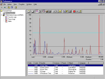
   Figure 8.18: Percentage-based Counters in System Monitor

9. Click the Add (+) button.

10. In the Performance object drop-down list, select Physical Disk:Disk Reads/sec.

11. In the Select instances from list box, select _Total, and then click Add.

12. Repeat steps 9, 10, and 11 to add the following counters:

    • Physical Disk:Disk Writes/sec

    • Physical Disk:Avg. Disk Queue Length

    • Memory:Available Bytes

    • Memory:Pages/sec

    • Processor:Interrupts/sec

    • Server Work Queues:Queue Length

    • System:Processor Queue Length

13. Click Close.

14. Your System Monitor window should look similar to Figure 8.19. Notice how busy the chart is beginning to look. Again, compare the scale of the counters to each other. Notice how several counters seem to stay at the bottom of the chart even though they are active. This illustrates that you should consider scale and try not to mix percentage-based counters with nonpercentage-based counters on the same graph.

    
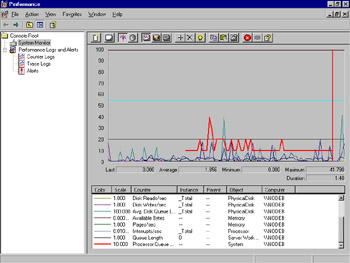
    Figure 8.19: All Common Counters in System Monitor

15. Click Logical Disk:%Free Space.

16. Click the Delete (X) button.

17. Repeat steps 9, 10, and 11 to add the following counters:

    • Physical Disk:%Disk Time

    • Logical Disk:%Disk Time

    • Paging File:%Usage

    • Processor:%Processor Time

18. You have removed all of the percentage-based counters from the graph. Your System Monitor window should appear similar to Figure 8.20. Compare the scale of the nonpercentage counters.

    
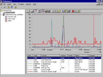
    Figure 8.20: Common Nonpercentage Counters

19. Close the Performance console.

Using Event Viewer to Monitor Servers

Windows Server 2003 includes several log files that collect information on events that occur in the system. Using these log files, you can view your system’s history of events. A standard Windows Server 2003 system has three event logs that record specific categories of events:

• Application Contains events generated by server-based applications, such as Microsoft Exchange and WINS. The specific events logged by each application are determined by the application itself and may be configurable by an administrator within the application.

• Security Contains events relating to system security, including successful and failed logon attempts, file creation or deletion, and user and group account activity. The contents of this file will vary depending on the auditing settings selected by the system administrator.

• System Contains events relating to the activity of the operating system. Startups and shutdowns, device driver events, and system service events are recorded in the System log. The configuration and installed options of the operating system determine the events recorded in this log. Because of the nature of its entries, this log is the most important for maintaining system health.

In addition to these three basic logs, a Windows Server 2003 system configured as a domain controller will also have the following two logs:

• Directory Service Contains events related to the operation of Active Directory (AD). AD database health, replication events, and Global Catalog activities are recorded in this log.

• File Replication Service Contains events related the File Replication Service (FRS), which is responsible for the replication of the file system-based portion of Group Policy Objects (GPOs) between domain controllers.

Finally, a server configured to run the DNS Server service will have the DNS Server log, which contains events related to the operations of that service. Client DNS messages are recorded in the System log.

Events entered into these log files occur as one of five different event types. The type of an event defines it level of severity. The five types of events are as follows:

• Error Indicates the most severe or dangerous type of event. The failure of a device driver or service to start or a failed procedure call to a dynamic link library (DLL) can generate this type of event. These events indicate problems that could lead to downtime and need to be resolved. The icon of an error event appears as a red circle with a white X in the middle.

• Warning Indicates a problem that is not necessarily an immediate issue but has the potential to become one. Low disk space is an example of a Warning event. This event type icon is a yellow triangle with a white exclamation point (!) in it.

• Information Usually indicates success. Proper loading of a driver or startup of a service will generate an Information event. This icon is a white message balloon with a blue, lowercase letter i in it.

• Success Audit In the Security log, indicates the successful completion of an event configured for security auditing. A successful logon will generate this event. This icon is a gold key.

• Failure Audit In the Security log, indicates the unsuccessful completion of an event configured for security auditing. An attempted logon with an incorrect password or an attempt to access a file without sufficient permissions will generate this type of event. The event’s icon is a locked padlock.

The event logs are very helpful for collecting data, but we need a tool to present, filter, search, and help us interpret the data. That tool is Event Viewer, shown in Figure 8.21, which can be accessed by selecting Start | All Programs | Administrative Tools | Event Viewer.

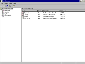
Figure 8.21: The Event Viewer Window

Event Viewer can also be accessed as a component of the System Tools snap-in within the Computer Management utility, as shown in Figure 8.22.

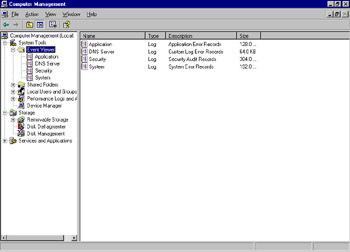
Figure 8.22: Event Viewer, as Viewed from Computer Management

When viewing an event log, the events appear in the order they occurred. Double-clicking an event will bring up the properties of that event, as shown in Figure 8.23. Click the arrows to navigate to either the next or previous event.

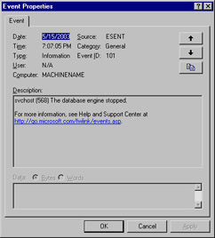
Figure 8.23: Viewing Event Properties

Each event captured follows the same format and contains the same set of data points. Those data points form the event header and are as follows:

• Date The date the event occurred.

• Time The time the event occurred.

• Type The applicable type of event (Error, Warning, and so on).

• User The user or account context that generated the event.

• Computer The name of the computer where the event occurred.

• Source The application or system component that generated the event.

• Category The classification of the event from the event source’s perspective.

• Event ID A number identifying the specific event from the source’s perspective.

• Description A textual description of the event. This may be in any readable structure.

• Data A hexadecimal representation of any data recorded for the event by the source.

An event log can contain thousands or even millions of events. Because the event header follows the same structure regardless of the event source, you can use the filter function to focus in on specific patterns of events. The filter function is available from the log’s Properties dialog box. Right-click a log in the left tree view and select Properties from the context menu, as shown in Figure 8.24, to view its properties.

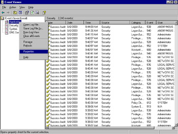
Figure 8.24: Accessing the Properties of an Event Log

Click the Filter tab to display the filter options, as shown in Figure 8.25. (You can also access the filter function by clicking View | Filter.)

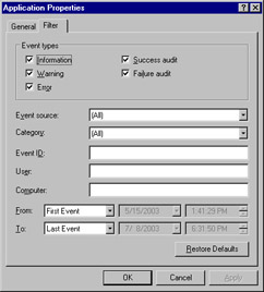
Figure 8.25: Filtering Event Log Data

By changing the selections on the Filter tab, you can exclude from view those events that do not fit the filter selections. Put another way, events that do not match the filter selections are filtered out. The events are still in the log; they are just not displayed as long as the filter is active. In addition to using the filter function, you can search event logs for specific events. From the Event Viewer main window, select View | Find…, as shown in Figure 8.26.

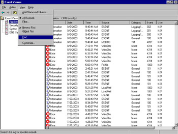
Figure 8.26: Using Find in an Event Log

In the Find dialog box, enter your criteria for the search and click the Find Next button. The next event that matches your criteria will be highlighted in the Event Viewer main window, as shown in the example in Figure 8.27.

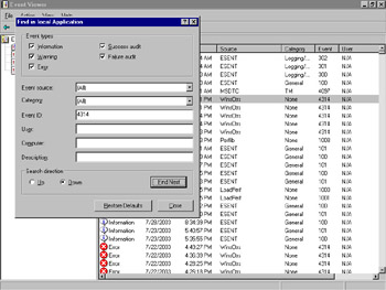
Figure 8.27: Finding Event Log Data

The event log files themselves are stored in a compact binary format in the %systemroot%\System32\Config directory. You can configure the maximum size of these files and what action is taken when this size is reached on the General tab of the log Properties dialog box, as shown in Figure 8.28.

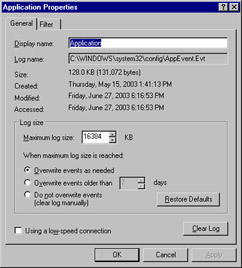
Figure 8.28: Event Log General Properties

Accessing the Properties dialog box of an event log gives you access to information about the log itself, and allows you to change certain characteristics of the log. Referring to Figure 8.28, you can see the log’s name, location, and size. The Maximum log size option allows you to limit the amount of space the log consumes. The three radio buttons below this option allow you to specify what will happen when this maximum size is reached.

Event logs can be archived on the computer on which they occur for long-term storage and analysis. This can be accomplished in two ways. The first is through the use of the Clear Log button on the event log Properties dialog box. You can click this button to delete all entries from a log file, but this process will also prompt you to save the events prior to deletion. The second method is through the use of the Save Log File As… option on the context menu for a log file, as shown in Figure 8.29.

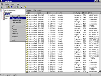
Figure 8.29: Saving a Log File, Selection Menu

The Save Log File As… selection brings up a Save AS dialog box, as shown in Figure 8.30, which allows you to choose the name, location, and format of the archive.

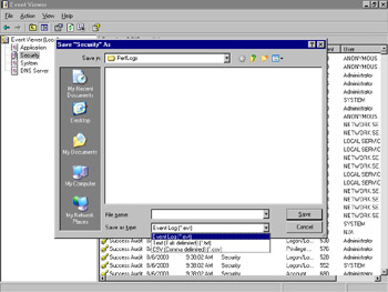
Figure 8.30: Saving a Log File

You can save events in a binary .evt, comma-delimited, or tab-delimited text file. You can use the .evt format to retain the log file in a compact format, which you can reopen in Event Viewer by selecting Action | Open Log File…, as shown in Figure 8.31. The delimited archive file formats consume more disk space than the .evt format, but they can be imported into a database or an application like Microsoft Excel for further analysis.

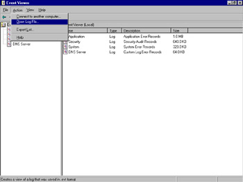
Figure 8.31: Opening an Archived Log File

Choosing to open a log file brings up an Open dialog box, shown in Figure 8.32. In this dialog box, you can locate and choose the archived file.

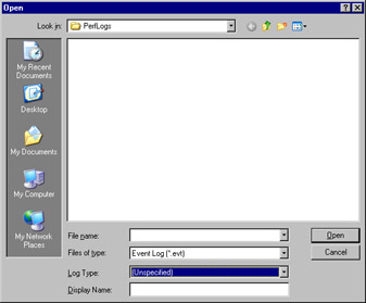
Figure 8.32: Selecting an Archived Event Log

Using Service Logs to Monitor Servers

As mentioned previously, there are additional event logs for servers in certain roles. A server running the DNS server will have a DNS Server log. A server acting as a domain controller will have logs for the Directory Service and File Replication Service. It is also possible that other services or applications may create their own log files, but most do not.

These server log files follow the same format as the other event logs. They can be filtered, searched, and archived using the methods described in the previous sections. These logs exist mainly to collect the events from these services in one place other than the System log. These services generate a greater number of events than do other services.