Section 7.6. Congestion Control at Network Layer

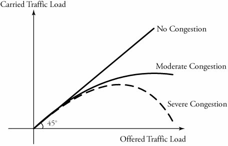
7.6. Congestion Control at Network Layer

Congestion represents an overloaded condition in a network. Congestion control can be achieved by optimum usage of the available resources in the network. Figure 7.11 shows a set of performance graphs for networks in which three possible cases are compared: no congestion, moderate congestion, and severe congestion. These plots indicate that if a network has no congestion control, the consequence may be a severe performance degradation, even to the extent that the carried load starts to fall with increasing offered load. The ideal situation is the one with no loss of data, as a result of no congestion, as shown in the figure. Normally, a significant amount of engineering effort is required to design a network with no congestion.

Figure 7.11. Comparison among networks in which congestion, moderate congestion, and severe congestion exist

Congestion can be either logical or physical , as shown in Figure 7.12. The queueing feature in two routers can create a logical bottleneck between user A and user B. Meanwhile, insufficient bandwidtha resource shortageon physical links between routers and the network can also be a bottleneck, resulting in congestion. Resource shortage can occur

At the link layer , where the link bandwidth runs out
At the network layer , where the queues of packets at nodes go out of control
At the transport layer , where logical links between two routers within a communication session go out of control

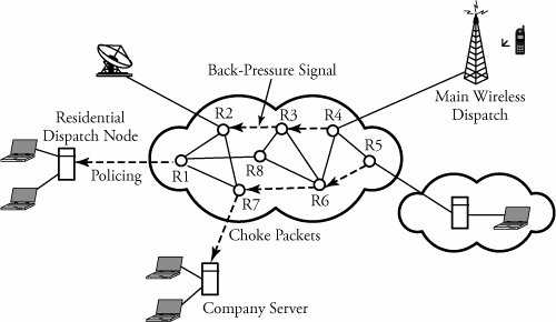
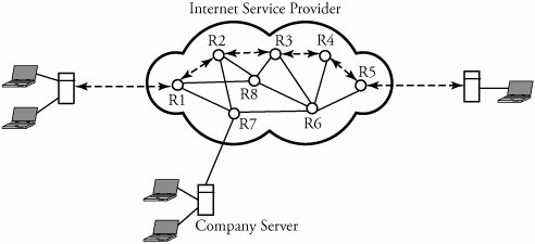
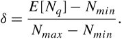
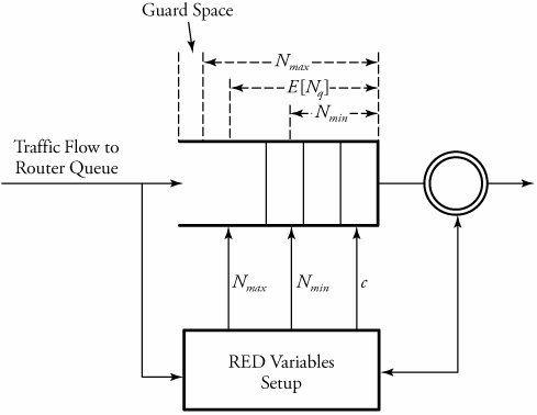
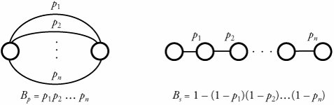
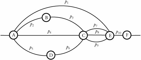
Figure 7.12. Forms of bottleneck along a round-trip path between two users

One key way to avoid congestion is to carefully allocate network resources to users and applications. Network resources, such as bandwidth and buffer space, can be allocated to competing applications. Devising optimum and fair resource-allocation schemes can control congestion to some extent. In particular, congestion control applies to controlling data flow among a group of senders and receivers, whereas flow control is specifically related to the arrangement of traffic flows on links. Both resource allocation and congestion control are not limited to any single level of the protocol hierarchy. Resource allocation occurs at switches, routers, and end hosts . A router can send information on its available resources so that an end host can reserve resources at the router to use for various applications.

General methods of congestion control are either unidirectional or bidirectional . These two schemes are described next .

7.6.1. Unidirectional Congestion Control

A network can be controlled unidirectionally through back-pressure signaling , transmission of choke packets , and traffic policing . Figure 7.13 shows a network of eight routers: R1 through R8. These routers connect a variety of servicing companies: cellphones, satellite, residential, and company LANs. In such a configuration, congestion among routing nodes may occur at certain hours of the day.

Figure 7.13. Unidirectional congestion control

The first type of congestion control is achieved by generating a back-pressure signal between two routers. The back-pressure scheme is similar to fluid flow in pipes. When one end of a pipe is closed, the pressure propagates backward to slow the flow of water at the source. The same concept can be applied to networks. When a node becomes congested , it slows down the traffic on its incoming links until the congestion is relieved. For example, in the figure, router R4 senses overloading traffic and consequently sends signals in the form of back-pressure packets to router R3 and thereby to router R2, which is assumed to be the source of overwhelming the path. Packet flow can be controlled on a hop-by-hop basis. Back-pressure signaling is propagated backward to each node along the path until the source node is reached. Accordingly, the source node restricts its packet flow, thereby reducing the congestion.

Choke-packet transmission is another solution to congestion. In this scheme, choke packets are sent to the source node by a congested node to restrict the flow of packets from the source node. A router or even an end host can send these packets when it is near full capacity, in anticipation of a condition leading to congestion at the router. The choke packets are sent periodically until congestion is relieved. On receipt of the choke packets, the source host reduces its traffic-generation rate until it stops receiving them.

The third method of congestion control is policing and is quite simple. An edge router, such as R1 in the figure, acts as a traffic police and directly monitors and controls its immediate connected consumers. In the figure, R1 is policing a residential dispatch node from which traffic from a certain residential area is flowing into the network.

7.6.2. Bidirectional Congestion Control

Figure 7.14 illustrates bidirectional congestion control , a host-based resource-allocation technique. The destination end host controls the rate at which it sends traffic, based on observable network conditions, such as delay and packet loss. If a source detects long delays and packet losses, it slows down its packet flow rate. All sources in the network adjust their packet-generation rate similarly; thus, congestion comes under control. Implicit signaling is widely used in packet-switched networks, such as the Internet.

Figure 7.14. Bidirectional congestion control

In bidirectional signaling, network routing nodes alert the source of congested resources by setting bits in the header of a packet intended for the source. An alternative mechanism for signaling is to send control packets as choke packets to the source, alerting it of any congested resources in the network. The source then slows down its rate of packet flow. When it receives a packet, the source checks for the bit that indicates congestion. If the bit is set along the path of packet flow, the source slows down its sending rate. Bidirectional signaling can also be imposed by the window-based and rate-based congestion-control schemes discussed earlier.

7.6.3. Random Early Detection (RED)

Random early detection (RED) avoids congestion by detecting and taking appropriate measures early. When packet queues in a router's buffer experience congestion, they discard all incoming packets that could not be kept in the buffer. This tail-drop policy leads to two serious problems: global synchronization of TCP sessions and prolonged congestion in the network. RED overcomes the disadvantages of the tail-drop policy in queues by randomly dropping the packets when the average queue size exceeds a given minimum threshold.

From the statistical standpoint, when a queueing buffer is full, the policy of random packet drop is better than multiple-packet drop at once. RED works as a feedback mechanism to inform TCP sessions that the source anticipates congestion and must reduce its transmission rate. The packet-drop probability is calculated based on the weight allocation on its flow. For example, heavy flows experience a larger number of dropped packets. The average queue size is computed, using an exponentially weighted moving average so that RED does not react to spontaneous transitions caused by bursty Internet traffic. When the average queue size exceeds the maximum threshold, all further incoming packets are discarded.

RED Setup at Routers

With RED, a router continually monitors its own queue length and available buffer space. When the buffer space begins to fill up and the router detects the possibility of congestion, it notifies the source implicitly by dropping a few packets from the source. The source detects this through a time-out period or a duplicate ACK. Consequently, the router drops packets earlier than it has to and thus implicitly notifies the source to reduce its congestion window size.

The "random" part of this method suggests that the router drops an arriving packet with some drop probability when the queue length exceeds a threshold. This scheme computes the average queue length, E [ N _q ], recursively by

Equation 7.3

where N _i is the instantaneous queue length, and 0 <± < 1 is the weight factor. The average queue length is used as a measure of load. The Internet has bursty traffic, and the instantaneous queue length may not be an accurate measure of the queue length. RED sets minimum and maximum thresholds on the queue length, N _min and N _max , respectively. A router applies the following scheme for deciding whether to service or drop a new packet. If E [ N _q ] N _max , any new arriving packet is dropped. If E [ N _q ] N _min , the packet is queued. If N _min < E [ N _q ] <N _max , the arriving packet is dropped with probability P given by

Equation 7.4

where coefficient c is set by the router to determine how quickly it wants to reach a desired P . In fact, c can be thought of as the number of arriving packets that have been queued. We can then obtain ƒ from

Equation 7.5

In essence, when the queue length is below the minimum threshold, the packet is admitted into the queue. Figure 7.15 shows the variable setup in RED congestion avoidance . When the queue length is between the two thresholds, the packet-drop probability increases as the queue length increases. When the queue length is above the maximum threshold, the packet is always dropped. Also, shown in Equation (7.4), the packet-drop probability depends on a variable that represents the number of arriving packets from a flow that has been queued. When the queue length increases , all that is needed is to drop one packet from the source. The source then halves its congestion window size.

Figure 7.15. Variables setup in the RED congestion-avoidance method

Once a small number of packets are dropped, the associated sources reduce their congestion windows if the average queue length exceeds the minimum threshold, and therefore the traffic to the router drops. With this method, any congestion is avoided by an early dropping of packets.

RED also has a certain amount of fairness associated with it; for larger flows, more packets are dropped, since P for these flows could become large. One of the challenges in RED is to set the optimum values for N _min , N _max , and c . Typically, N _min has to be set large enough to keep the throughput at a reasonably high level but low enough to avoid congestion. In practice, for most networks on the Internet, the N _max is set to twice the minimum threshold value. Also, as shown by guard space in Figure 7.15, there has to be enough buffer space beyond N _max , as Internet traffic is bursty.

7.6.4. A Quick Estimation of Link Blocking

A number of techniques can be used to evaluate a communication network's blocking probabilities. These techniques can vary according to accuracy and to network architectures. One of the most interesting and relatively simple approaches to calculating the level of blocking involves the use of Lee's probability graphs. Although Lee's technique requires approximations, it nonetheless provides reasonably accurate results.

Serial and Parallel Connection Rules

Lee's method is based on two fundamental rules of serial and parallel connections. Each link is represented by its blocking probability, and the entire network of links is evaluated, based on blocking probabilities represented on each link, using one or both of the rules. This approach is easy to formulate , and the formula directly relates to the underlying network structures, without requiring any other detailed parameters. Thus, Lee's approach provides insight into the network structures, giving a remarkable solution for performance evaluations.

Let p be the probability that a link is busy, or the percentage of link utilization. Thus, the probability that a link is idle is denoted by q = 1 - p . Now, consider a simple case of two links in parallel to complete a connection with probabilities p ₁ and p ₂ . The composite blocking probability, B _p , is the probability that both links are in use, or

Equation 7.6

If these two links are in series to complete a connection, the blocking probability, B _s , is determined as 1 minus the probability that both links are available:

Equation 7.7

We can generalize the estimation of a network of links by two fundamental rules.

Rule 1: For a parallel connection of links, the blocking probability is estimated by forming the product of the blocking probabilities for the subnetworks, as shown in Figure 7.16. Let a source and a destination be connected in general through n links with probabilities p ₁ through p _n , respectively, as shown in Figure 7.16. Therefore, if the source and the destination are linked through parallel connections, the probability of blocking B _p is obtained from a product form as follows :

Equation 7.8

Figure 7.16. Models for serial and parallel connection rules
Rule 2: For a serial connection of links, the probability of blocking is estimated by forming the product of the probabilities of no blocking for the network. This method makes the assumption that the probability that a given link is busy is independent from link to link. Although this independence assumption is not strictly correct, the resulting estimates are sufficiently accurate. If links are in series, the probability of blocking is obtained from

Equation 7.9

Example.

The network in Figure 7.17 has six nodes, A through F, interconnected with ten links. The corresponding blocking probabilities of links, p ₁ through p ₁₀ , are indicated on the corresponding links. For this network, find the overall blocking probability from A to F.

Figure 7.17. A network of links and their blocking probabilities

Solution.

This network consists of a number of serial and parallel connections: for example, p _ADC = 1 - (1 - p ₅ )(1 - p ₆ ), p _ABC = 1 - (1 - p ₂ )(1 - p ₃ ), and p _CE = p ₇ p ₈ p ₉ . Thus:

B = p _AF = 1 - {1 - [1 - (1 - p ₄ . p _ABC . p _ADC )( 1 - p _CE ) ] p ₁ } (1 - p ₁₀ ).