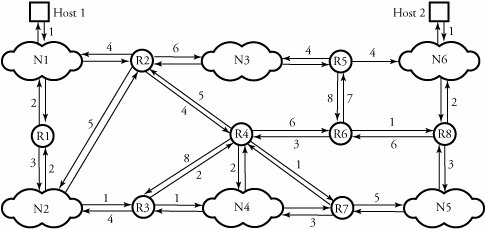
Section 7.4. Intradomain Routing Protocols | Computer and Communication Networks (paperback)

7.4. Intradomain Routing Protocols

There are two classes of routing protocols: intradomain routing protocol or intranetwork routing protocol or intranet , and interdomain routing protocol or internetwork routing protocol or extranet . An intradomain routing protocol routes packets within a defined domain, such as for routing e-mail or Web browsing within an institutional network. By contrast, an interdomain routing protocol is a procedure for routing packets on networks of domains and is discussed in Section 7.5.

Figure 7.5 shows intradomain routing; each point-to-point link connects an associated pair of routers and indicates the corresponding cost of the connection. A host is an end system that can be directly connected to the router. A cost is considered with the output side of each router interface. When nothing is written on an arrow, no cost is associated with that connection. An arrow that connects a network and a router has a zero cost. A database is gathered from each router, including costs of paths in all separate directions. In the figure, two hosts within a domain are exchanging data facing their own LANs (N1 and N6), several other LANs (N2 through N5), and several routers (R1 through R8).

Figure 7.5. Intradomain routing, with two hosts in a large domain exchanging data facing several LANs and routers

The most widely used intranetworking routing protocols are the two unicast routing protocols RIP and OSPF.

7.4.1. Routing Information Protocol (RIP)

The routing information protocol (RIP) is a simple intradomain routing protocol. RIP is one of the most widely used routing protocols in the Internet infrastructure but is also appropriate for routing in smaller domains. In RIP, routers exchange information about reachable networks and the number of hops and associated costs required to reach a destination. This protocol is summarized as follows .

Begin RIP Algorithm

Apply the Bellman-Ford algorithm in a distributed fashion, including all hosts and routers.
For each router, form an optimum vector of distance indicating the cost of routing and other necessary parameters, using distance-vector routing (discussed next ).
If a cost of routing at any point changes, propagate the change periodically to the neighboring routers and hosts of that point.
Update tables of routers and hosts periodically.

Table 7.3 shows routing information maintained in router R1 of the network shown in Figure 7.5. For example, at the third row of the routing table, the path to N3 is initiated through router R2 and established through path R1-N2-R2-N3, with a total cost of 8. Because routers and hosts within the network use vectors of data, a technique called distance vector routing is used.

Table 7.3. A routing table in router R1 in Figure 7.5a, using RIP

Destination Network	Next Router	Path	Cost
N1		R1-N1	2
N2		R1-N2	3
N3	R2	R1-N2-R2-N3	8
N4	R3	R1-N2-R3-N4	4
N5	R3	R1-N2-R3-N4-R7-N5	9
N6	R2	R1-N2-R3-N4-R7-N5-R8-N6	11

Distance Vector Routing

The distance vector algorithm was designed mainly for small network topologies. The term distance vector derives from the fact that the protocol includes its routing updates with a vector of distances, or hop counts. In distance vector routing, all nodes exchange information only with their neighboring nodes. Nodes participating in the same local network are considered neighboring nodes. In this protocol, each individual node i maintains three vectors:

B _i	=	[ b _i _,1 , ..., b _i _{, n} ] = link-cost vector
D _i	=	[ d _i _,1 , ..., d _i _{, m} ]= distance vector
H _i	=	[ h _i _,1 , ..., h _i _{, m} ]= next-hop vector

For the calculation of the link-cost vector, we consider node i to be directly connected to n networks out of the total of m existing networks. The link-cost vector B _i is a vector containing the costs of node i to its directly connected network. For example, b _i _,1 refers to the cost of node i to network 1. Distance vector D _i contains the estimated minimum delays from node i to all networks within its domain. For example, d _i _,1 is the estimated minimum delay from node i to network 1. Finally, the next-hop vector H _i is a matrix vector containing the next node in the minimum-delay path from node i to its directly connected network. As an example for this vector, h _i _,1 refers to the next node in the minimum-delay path from node i to Network 1. Each node exchanges its distance every r seconds with all its neighbors. Node i is responsible for updating both of its vectors by:

Equation 7.1

and

Equation 7.2

where {1, ..., n } is the set of network nodes for node i , and g(x , y ) is a network that connects node x to node y ; thus, b _i _{, g(x , y} ) is the cost of node i to network g(x , y ). Equations (7.1) and (7.2) are a distributed version of the Bellman-Ford algorithm, which is used in RIP. Each router i begins with d _i _, _j = b _i _, _j if it is directly connected to network j . All routers concurrently replace the distance vectors and compute Equation (7.1). Routers repeat this process again. Each iteration is equal to one iteration of step 2 in the Bellman-Ford algorithm, processed in parallel at each node of the graph. The shortest-length paths with a distance of at most one hop are considered after the first iteration. Then, the second iteration takes place, with the least-cost paths with at most two hops; this continues until all least-cost paths have been discovered .

Updating Routing Tables in RIP

Since RIP depends on distance vector routing, each router transmits its distance-vector to its neighbors. Normally, updates are sent as a replies whether or not requested . When a router broadcasts an RIP request packet, each router in the corresponding domain receiving the request immediately transmits a reply. A node within a short window of time receives distance-vectors from all its neighbors, and the total update occurs, based on incoming vectors. But this process is not practical, since the algorithm is asynchronous, implying that updates may not be received within any specified window of time.

RIP packets are sent typically in UDP fashion, so packet loss is always possible. In such environments, RIP is used to update routing tables after processing each distance vector. To update a routing table, if an incoming distance vector contains a new destination network, this information is added to the routing table. A node receiving a route with a smaller delay immediately replaces the previous route. Under certain conditions, such as after a router reset, the router can receive all the entries of its next hop to reproduce its new table.

The RIP split-horizon rule asserts that it is not practical to send information about a route back in the direction from which it was received. The split-horizon advantage is increased speed and removal of incorrect route within a timeout. The RIP poisoned-reverse rule has a faster response and bigger message size . Despite the original split horizon, a node sends updates to neighbors with a hop count of 16 for routing information arrived from those neighbors.

RIP Packet Format

Figure 7.6 shows the packet format of an RIP header. Each packet consists of several address distances. The header format contains the following specifications for the first address distance.

Command indicates a request with value 1 or a reply with value 2.
Version number specifies the version: RIP-1 or RIP-2.
Address family identifier shows the type of address, such as an IP address.
IP address provides the IP address in a particular network.
Metric identifies the distance from a router to a specified network.

Figure 7.6. Routing Information Protocol (RIP) header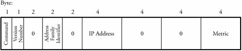

If a link cost is set to 1, the metric field acts as a hop count. But if link costs have larger values, the number of hops becomes smaller. Each packet consists of several address distances. If more than one address distance is needed, the header shown in Figure 7.6 can be extended to as many address distances as are requested, except for the command and version number and its 2 bytes of 0s; the remaining field structure can be repeated for each address distance.

Example.

Apply RIP for connecting Host 1 to all six networks in Figure 7.5, given that at a certain time, the cost of R2-N2 changes from 5 to 1, and the cost of R4-R6 changes from 6 to 2.

Solution.

The current routing table for the host is shown in Table 7.4. In particular, note the status of the table on destination network N2, where the next router is R1 with path Host1-N1-R1-N2 and a cost of 4. Changes on the link costs affect the status of the N2 and N6 entries. The new updates are reflected in Table 7.4, where the new path becomes Host1-R2-N2, with a new, lower cost of 2. The status of N6 also changes to a new path, Host1-R2-R4-R6-R8-N6, with a new, lower cost of 9.

Table 7.4. Current routing table with updated values for Host 1 in Figure 7.5, using RIP

Destination Network	Next Router	Cost	Updated Next Router	Updated Cost
N1		1		1
N2	R1	4	R2	2
N3	R2	7	R2	7
N4	R1	8	R1	8
N5	R2	11	R2	11
N6	R2	13	R2	9

Issues and Limitations of RIP

One of the disadvantages of RIP is its slow convergence in response to a change in topology. Convergence refers to the point in time at which the entire network becomes updated. In large networks, a routing table exchanged between routers becomes very large and difficult to maintain, which may lead to an even slower convergence. Also, RIP might lead to suboptimal routes, since its decision is based on hop counts. Thus, low-speed links are treated equally or sometimes preferred over high-speed links. Another issue with RIP is the count-to-infinity restriction. Distance vector protocols have a limit on the number of hops after which a route is considered inaccessible. This restriction would cause issues for large networks.

Other issues with RIP stem from the distance vector algorithm. First, reliance on hop counts is one deficiency, as is the fact that routers exchange all the network values via periodic broadcasts of the entire routing table. Also, the distance vector algorithm may cause loops and delays, since they are based on periodic updates. For example, a route may go into a hold state if the corresponding update information is not received in a certain amount of time. This situation can translate into a significant amount of delay in update convergence in the network before the network discovers that route information has been lost.

Another major deficiency is the lack of support for variable-length subnet masks. RIP does not exchange mask information when it sends routing updates. A router receiving a routing update uses its locally defined subnet mask for the update, which would lead to complications and misinterpretation in a variably subnetted network. Distance vector networks do not have hierarchies, which makes them incapable of integrating to larger networks.

7.4.2. Open Shortest Path First (OSPF)

The limitations of RIP make it a nonpreferred routing strategy as networks scale up. The Open Shortest Path First (OSPF) protocol is a better choice of intradomain routing protocols, especially for TCP/IP applications. OSPF is based on Dijikstra's algorithm, using a tree that describes the network topology to define the shortest path from each router to each destination address. Since it keeps track of all paths of a route, OSPF has more overhead than RIP, but provides more stability and useful options. The essence of this protocol is as follows.

Begin OSPF Protocol

Apply Dijikstra's algorithm or another efficient algorithm in a distributed fashion for each host and router.
In each host or router, calculate the least-cost path, and propagate it to all nodes, using link-state routing .
Periodically propagate any changes in routing cost to all routers and hosts.
Update the routing tables of routers and hosts.

Before focusing on the details of OSPF, we need to describe the essence of the link-state routing protocol.

Link-State Routing

In the link-state routing , routers collaborate by exchanging packets carrying status information about their adjacent links. A router collects all the packets and determines the network topology, thereby executing its own shortest-route algorithm.

As explained in the section on RIP, with distance vector routing, each router must send a distance vector to all its neighbors. If a link cost changes, it may take a significant amount of time to spread the change throughout the network. Link-state routing is designed to resolve this issue; each router sends routing information to all routers, not only to the neighbors. That way, the transmitting router discovers link-cost changes, so a new link cost is formed . Since each router receives all link costs from all routers, it is able to calculate the least-cost path to each destination of the network. The router can use any efficient routing algorithm, such as Dijkstra's algorithm, to find the shortest path.

The core function of the link-state algorithm is flood routing, which requires no network topology information. Let's review the three important properties of flooding used in link-state routing. First, a packet always traverses completely between a source and a destination, given at least one path between these two nodes. This property makes this routing technique robust. Second, at least one copy of the packet arriving at the destination must possess the minimum delay, since all routers in the network are tried. This property makes the flooded information propagate to all routers very quickly. Third, all nodes in the network are visited whether they are directly or indirectly connected to the source node. This property makes every router receive all the information needed to update its routing table.

Details of OSPF Operation

To return to the OSPF operation: Every router using OSPF is aware of its local link-cost status and periodically sends updates to all routers. After receiving update packets, each router is responsible for informing its sending router of receipt of the update. These communications, though, result in additional traffic, potentially leading to congestion. OSPF can provide a flexible link-cost rule based of type of service (TOS). The TOS information allows OSPF to select different routes for IP packets, based on the value of the TOS field. Therefore, instead of assigning a cost to a link, it is possible to assign different values of cost to a link, depending on the TOS the value for each block of data.

Figure 7.7. OSPF header format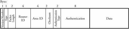

TOS has five levels of values: level 1 TOS, with the highest value to act by default, through level 5 TOS, with the lowest value for minimized delay. By looking at these five categories, it is obvious that a router can build up to five routing tables for each TOS. For example, if a link looks good for delay-sensitive traffic, a router gives it a low, level 5 TOS value for low delay and a high, level 2 TOS value for all other traffic types. Thus, OSPF selects a different shortest path if the incoming packet is normal and does not require an optimal route.

OSPF Packet Format

An IP packet that contains OSPF has a standard broadcast IP address of 224.0.0.5 for flood routing. All OSPF packets use a 24-byte header as follows:

Version number indicates the version of OSPF.
Type is one of the five types of packets for OSPF to choose from: hello , database description , link-state request , link-state update , and link-state acknowledgment .
Packet length specifies the length of the OSPF packet.
Router ID specifies the packet's source router ID.
Area ID refers to the area that the source router belongs to.
Checksum specifies the standard IP checksum of the packet contents (see Chapter 4).
Authentication type identifies which authentication method to choose (see Section 10.5).
Authentication specifies the authentication method (see Section 10.5).

The hello packet specified in the Type field is used to detect each router's active neighbors. Each router periodically sends out hello packets to its neighbors to discover its active neighboring routers. Each packet contains the identity of the neighboring router interface taken from the hello packet already received from it. The database description packets are used for database structure exchange between two adjacent routers to synchronize their knowledge of network topology. The link-state request packet is transmitted to request a specific portion of link-state database from a neighboring router. The link-state update packet transfers the link-state information to all neighboring routers. Finally, the link-state acknowledgment packet acknowledges the update of a link-state packet.

In summary, when a router is turned on, it transmits hello packets to all neighboring routers and then establishes routing connections by synchronizing databases. Periodically, each router sends a link-state update message describing its routing database to all other routers. Therefore, all routers have the same description of the topology of the local network. Every router calculates a shortest-path tree that describes the shortest path to each destination address, thereby indicating the closest router for communications.