Section 17.5. Limits of Compression with Loss

17.5. Limits of Compression with Loss

Hartely, Nyquist, and Shannon are the founders of information theory , which has resulted in the mathematical modeling of information sources. Consider a communication system in which a source signal is processed to produce sequences of n words, as shown in Figure 17.10. These sequences of digital bits at the output of the information source can be compressed in the source encoder unit to save the transmission link bandwidth. An information source can be modeled by a random process X _n = ( X ₁ , ..., X _n ) , where X _i is a random variable taking on values from a set of values as { a ₁ , ...,a _N }, called alphabet . We use this model in our analysis to show the information process in high-speed networks.

Figure 17.10. A model of data sequences

17.5.1. Basics of Information Theory

The challenge of data compression is to find the output that conveys the most information. Consider a single source with random variable X , choosing values in { a ₁ , ... a _N }.

If a _i is the most likely output and a _j is the least likely output, clearly, a _j conveys the most information and a _i conveys the least information. This observation can be rephrased as an important conclusion: The measure of information for an output is a decreasing and continuous function of the probability of source output . To formulate this statement, let P _{k 1} and P _{k 2} be the probabilities of an information source's outputs a _{k 1} and a _{k 2} , respectively. Let I(P _{k 1} ) and I(P _{k 2} ) be the information content of a _{k 1} and a _{k 2} , respectively. The following four facts apply.

1. As discussed, I(P _k ) depends on P _k .

2. I(P _k ) = a continuous function of P _k .

3. I(P _k ) = a decreasing function of P _k .

4. P _k = P _{k 1} . P _{k 2} (probability of two outputs happen in the same time).

5. I(P _k ) = I(P _{k 1} ) + I(P _{k 2} ) (sum of two pieces of information).

These facts lead to an important conclusion that can relate the probability of a certain data to its information content:

Equation 17.16

The log function has a base 2, an indication of incorporating the binary concept of digital data.

17.5.2. Entropy of Information

In general, entropy is a measure of uncertainty. Consider an information source producing random numbers , X , from a possible collection of { a ₁ , ..., a _N } with corresponding probabilities of { P ₁ ,...,P _N } and information content of { I (P ₁ ),..., I (P _N )}, respectively. In particular, the entropy, H(x) , is defined as the average information content of a source:

Equation 17.17

Example.	A source with bandwidth 8 KHz is sampled at the Nyquist rate. If the result is modeled using any value from {-2,-1,0,1,2} and corresponding probabilities {0.05, 0.05, 0.08, 0.30, 0.52}, find the entropy.
Solution.

The information rate in samples/sec = 8,000 x 2 = 16,000, and the rate of information produced by the source = 16,000 x 0.522 = 8,352 bits.

Joint Entropy

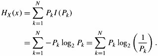
The joint entropy of two discrete random variables X and Y is defined by

Equation 17.18

where P _X,Y ( x , y ) = Prob[ X = x and the same time Y = y ] and is called the joint probability mass function of two random variables. In general, for a random process X _n = ( X ₁ ,..., X _n ) with n random variables:

Equation 17.19

where P _{X1, ..., Xn} ( x ₁ , ...., x _n ) is the joint probability mass function (J-PMF) of the random process X _n . For more information on J-PMF, see Appendix C.

17.5.3. Shannon's Coding Theorem

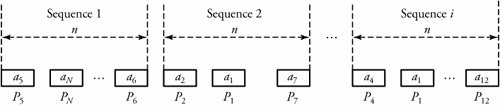
This theorem limits the rate of data compression. Consider again Figure 17.10, which shows a discrete source modeled by a random process that generates sequences of length n using values in set { a ₁ , ..., a _N } with probabilities { P ₁ , ..., P _N }, respectively. If n is large enough, the number of times a value a _i is repeated in a given sequence = nP _i , and the number of values in a typical sequence is therefore n(P ₁ +... + P _N ) .

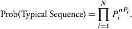
We define the typical sequence as one in which any value a _i is repeated nP _i times. Accordingly, the probability that a _i is repeated nP _i times is obviously , resulting in a more general statement: The probability of a typical sequence is the probability [( a ₁ is repeated np ₁ )] x the probability [( a ₂ is repeated np ₂ ] x .... This can be shown by , or

Equation 17.20

Knowing , we can obtain the probability of a typical sequence P _t as follow:

Equation 17.21

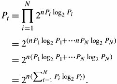
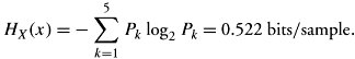
This last expression results in the well-known Shannon's theorem, which expresses the probability that a typical sequence of length n with entropy H _X (x) is equal to

Equation 17.22

Example.

Assume that a sequence size of 200 of an information source chooses values from the set { a 1 , ..., a 5 } with corresponding probabilities {0.05, 0.05, 0.08, 0.30, 0.52}. Find the probability of a typical sequence.

Solution.

In the previous example, we calculated the entropy to be H X (x) = 0.522 for the same situation. With n = 200, N = 5, the probability of a typical sequence is the probability of a sequence in which a 1 , a 2 , a 3 , a 4 , and a 5 are repeated, respectively, 200 x 0.05 = 10 times, 10 times, 16 times, 60 times, and 104 times. Thus, the probability of a typical sequence is P t = 2 -nH X (x) = 2 -200(0.52) .

The fundamental Shannon's theorem leads to an important conclusion. As the probability of a typical sequence is 2 ^- nH _X (x) and the sum of probabilities of all typical sequences is 1, the number of typical sequences is obtained by .

Knowing that the total number of all sequences, including typical and nontypical ones, is N ⁿ , it is sufficient, in all practical cases when n is large enough, to transmit only the set of typical sequences rather than the set of all sequences. This is the essence of data compression: The total number of bits required to represent 2 ^nH X(x) sequences is nH _X (x) bits, and the average number of bits for each source = H _X (x) .

Example.	Following the previous example, in which the sequence size for an information source is 200, find the ratio of the number of typical sequences to the number of all types of sequences.
Solution.	We had n = 200 and N = 5; thus, the number of typical sequences is 2 nH (x) =2 200 x0.522, and the total number of all sequences is 5 200 . This ratio is almost zero, which may cause a significant loss of data if it is compressed, based on Shannon's theorem. It is worth mentioning that the number of bits required to represent 2 nH X (x) sequences is nH X (x) = 104 bits.

17.5.4. Compression Ratio and Code Efficiency

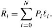
Let be the average length of codes, _i be the length of code word i , and P _i be the probability of code word i :

Equation 17.23

A compression ratio is defined as

Equation 17.24

where _x is the length of a source output before coding. It can also be shown that

Equation 17.25

Code efficiency is a measure for understanding how close code lengths are to the corresponding decoded data and is defined by

Equation 17.26

When data is compressed, part of the data may need to be removed in the process.