Section 13.8. Case Study: Multipath Buffered Crossbar

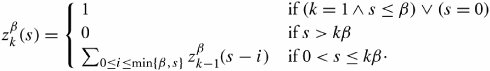
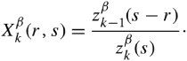
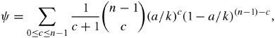
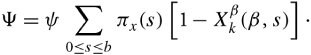
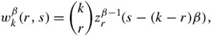
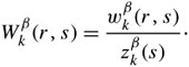
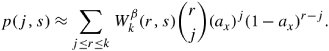
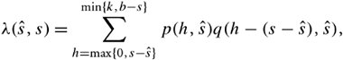
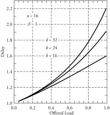
13.8. Case Study: Multipath Buffered Crossbar

For our case study on a switching fabric, we choose an expandable switch fabric constructed with identical building-block modules called the multipath buffered crossbar (MBC). Conventional n x n crossbars are vulnerable to faults. Unlike a conventional crossbar, MBC is a crossbar with n rows and k columns . Each row contains an input bus and an output bus. A packet being transferred from input i to output j is sent by input port processor i on input bus i to one of the k columns. The packet then passes along this column to the output bus in row j . The crosspoints that make up the MBC switch fabric include mechanisms that allow the inputs to contend for access to the various columns. The crosspoint buffers in one row act as a distributed output buffer for the corresponding output port. As shown in Figure 13.13, every crosspoint has two different switches and a buffer.

Figure 13.13. Routing and multicasting in the multipath buffered crossbar ( n = k = 4)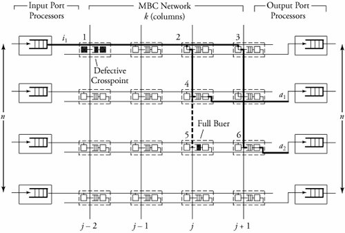

Consider a case of point-to-point connection from input i ₁ to output a ₁ . The packet is first randomly sent to a crosspoint at one of the k shared data buses , say, column ( j - 2). In case the crosspoint on this bus is not available for any reason, another crosspoint selected at random is examined, and so on. The reason for randomizing the initial location is to distribute the traffic as evenly as possible. When a functioning crosspoint (crosspoint 3) at column j is selected, the packet can be sent to a second crosspoint (crosspoint 4) at this column unless the selected crosspoint is found to be faulty or its buffer is full. The packet is buffered in crosspoint 4 and can be sent out after a contention -resolution process in its row.

The availability of each crosspoint at a given node ( i , j ) is dynamically reported to the input ports by a flag g _{i , j} . If more than one input port requests a given column, based on a contention-resolution process, only one of them can use the column. Packets in the other input ports receive higher priorities to examine other columns. Obviously, the more the packet receives priority increments , the sooner it is granted one free column, which it selects randomly. Once it gets accepted by one of the ² buffers of a second crosspoint, the packet contends to get access to its corresponding output. The losers of the contention resolution get higher priorities for the next contention cycle until they are successfully transmitted. In Figure 13.13, the connections i ₁ a ₁ and i ₁ a ₂ are made possible through nodes {2, 4} and nodes {3, 6}, respectively.

13.8.1. Queueing Model

The queueing model for this system is shown in Figure 13.14. Packets enter the network from n input port buffers and pass through any of the k crosspoints belonging to the same row as the input. These crosspoints do not contribute in any queueing operation and act only as ordinary connectors. Each packet exiting these nodes can confront n crosspoint buffers of length ² that are situated on one of the k -specified columns. A packet selects a buffer on the basis of the desired address. In this system architecture, each crossbar row contains k buffers, constructing a related group of buffers called a queue set , as seen in the figure. The winning packet of each set is then permitted to enter the corresponding output port buffer .

Figure 13.14. Queueing model for multipath buffered crossbar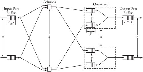

Note that the state of a buffer within each queue set is dependent on the state of all other buffers in that queue set. There are no grant flows between the output port buffers and the crosspoint buffers, and the admission of a packet by a queue set is made possible by granting the flag acknowledgments to the input port buffers. It should also be noted that the analysis that follows assumes that all crosspoints are functional. Let z ^² _k (s) be the number of ways to distribute s packets among k distinct buffers within a queue set, under the restriction that each buffer may contain at most ² packets. Note that here, we are not concerned about the number of combinations of different packets in the queue. Therefore, can be recursively computed by

Equation 13.20

Let be the probability that a given crosspoint buffer has r packets when the entire queue set contains s packets. Then

Equation 13.21

To further extend this analysis, an expression for the flow control between a crosspoint queue set and the input buffers is required. A second crosspoint generates a final flag acknowledgment, , after having completed a three-step process. The probability that a packet is available to enter the network, a , is the same probability that the input port buffer is not empty and is given by

Equation 13.22

Let ˆ be the probability that a packet contending for access to a column wins the contention. Note that the probability that any given input attempts to contend for any given column is a/k . Hence,

Equation 13.23

where is a binomial coefficient indicating the number of different combinations of n - 1 possible existing contenders on one of the k columns, taken c contenders at a time. Now, the probability that a packet forwarded by input port buffer i is admitted,, is given by:

Equation 13.24

We use later to derive the probability that an input port buffer contains exactly a certain number of packets.

13.8.2. Markov Chain Model

The expression for facilitates the determination of the state of the input port buffers. The input port queue can be modeled as a (2 ± + 1)-state Markov chain (see Figure 13.15). The transition rates are determined by the offered load and the crosspoint queue-set grant probability . Let f be the probability that a packet has fanout 2 (a bipoint connection ). In this model, a bipoint connection, which is a two-copying packet-recirculation task, is treated as two independent point-to-point connections. The upper row of the Markov chain depicts the state of the queue when a packet needs no additional copy. However, if the packet has fanout 2, it proceeds to the second copy of the packet on the upper row once the operation for its first copy in the lower row of the chain is completed.

Figure 13.15. Markov chain model of the input port queue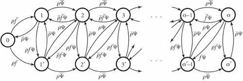

The state of the queue can be changed from 0 to 1 with transition probability if the packet has fanout 1, or it can enter state 1 ^' with transition probability f if the packet has fanout 2. On the arrival of a fanout-2 packet at the head of queue, a state in the upper chain is changed to a lower one with probability of f if a new packet arrives at the queue, or if no new packet arrives. Similarly, any of the lower chain states can be changed with probabilities or to an upper one as soon as the first copy of a fanout-2 packet is completed. These transition probabilities are free of f , since only the first copy has been completed at this point. The second copy is processed in the upper chain independently. The probability that an input port buffer contains exactly s packets is computed recursively by

Equation 13.25

and

Equation 13.26

Next, let be the number of distributions that leave exactly r buffers of capacity ² "not full" while a queue set contains s packets, and let be the probability that exactly r buffers are not full when a queue set contains s packets. Therefore:

Equation 13.27

and then,

Equation 13.28

Now, we need to compute the probability that exactly j packets enter a queue set when the queue is in state s at the beginning of the current packet cycle. The probability that a packet is available to enter a particular buffer of a queue set, a _x , is calculated based on a that was introduced earlier and is given by

Equation 13.29

Then, p(j , s ) is

Equation 13.30

We also need to compute the probability that exactly j packets leave a queue set when the queue is in state s at the beginning of the current packet cycle. It should be remembered that for q(j , s ), there is only one output for every queue set, owing to the queueing model, so the probability is introduced by a simple form of

Equation 13.31

Each queue set is modeled as a ( b + 1)-state Markov chain ( b = k² ). The transition probability, »( , s ), and the next-state probability, _x (s) , defined earlier, can be determined as follows:

Equation 13.32

where 0 ( s and ) b , and

Equation 13.33

By having _x (s) , we can estimate the system delay and throughput.

13.8.3. Throughput and Delay

By putting together all the preceding parameters, we can compute the system throughput ( T ) and delay ( D ). The throughput refers to the number of packets leaving a queue set per output link per packet cycle. Since the entire network is modeled as one middle-stage queue, the throughput, on the other hand, is the probability of having at least one packet in a queue set and is simply

Equation 13.34

Clearly, from the definition given by Equation (13.31), q(j , s ) ˆˆ {0, 1}. Thus, so long as at least one packet is in the queue set, q(j , s ) = 1, and T can be expressed free of q(j , s ). The delay is defined as the number of packet cycles that a given packet spends in the crossbar from network entry until network exit. This is another interpretation of the ratio of queue length and the arrival rate . Let the queue length of the network and the input port processors be denoted by Q _x and Q _i , respectively. They are expressed by

Equation 13.35

and

Equation 13.36

The arrival rate at the input port buffers is the offered load, , and the arrival rate for each queue set can be defined by A :

Equation 13.37

Thus, the total delay is the summation of the delays:

Equation 13.38

The delay ( D ) measurement is based on three main variables : , n , and k . Figure 13.16 shows a set of results. This figure shows variations of incoming traffic load on a 16-port MBC network. In these examples, ² = 1, and the fraction of multipoint packets is assumed to be f = 0.75. As expected, the throughput is improved when k increases as 16, 24, 32, mainly because of the availability of a larger number of columns for packets waiting in the input buffers. Delay curves show that the average time that packets spend in the network cannot exceed 2.2 packet times. This amount of time was predictable, since packets pass through only two stages of switching from an input port to their destinations. This behavior explains the better performance capability of an MBC switch fabric compared to a typical multistage switch fabric.