Section 11.5. Non-Markovian and Self-Similar Models

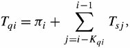
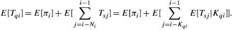
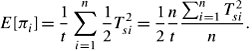
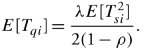
11.5. Non-Markovian and Self-Similar Models

Another class of queueing systems is either completely or partially non-Markovian . Partial non-Markovian means that either arrival or service behavior is not based on Markovian models. We first consider a single server in which packets arrive according to a Poisson process, but the service-time distribution is non-Poisson or non-Markovian as general distribution . One example of a non-Markovian system is M/G/ 1 queues with priorities. Another is M/D/ 1, where the distribution of service time is deterministic, not random. Yet another example is reservation systems in which part of the service time is occupied with sending packetsserving packetsand part with sending control information or making reservations for sending the packets.

11.5.1. Pollaczek-Khinchin Formula and M/G/1

Let us consider a single-server scenario in which packets arrive according to a Poisson process with rate » , but packet service times have a general distribution . This means that the distribution of service times cannot necessarily be exponential, as shown in Figure 11.16. Suppose that packets are served in the order they are received, with T _si the service time of the i th packet. In our analysis, we assume that random variables T _{s 1} , T _{s 2} , ... are identically distributed, mutually independent, and independent of the interarrival times. Let T _qi be the queueing time of the i th packet. Then:

Equation 11.50

Figure 11.16. A general distribution of service times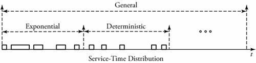

where K _qi is the number of packets found by the i th packet waiting in the queue on arrival, and _i is the partial service time seen by the i th packet if a given packet j is already being served when packet i arrives. If no packet is in service, _i is zero. In order to understand the averages of the mentioned times, we take expectations of two sides in Equation (11.50):

Equation 11.51

With the independence induction of the random variables K _qi and T _qj , we have

Equation 11.52

It is clear that we can apply the average service time as E [ T _si ] = 1/¼ in Equation (11.52). Also, by forcing Little's formula, where E [ K _qi ] = »E [ T _qi ], Equation (11.52) becomes

Equation 11.53

where = »/ µ is the utilization. Thus,

Equation 11.54

Figure 11.17 shows an example of mean _i representing the remaining time for the completion of an in-service packet as a function of time. If a new service of T _si seconds begins, _i starts at value T _si and decays linearly at 45 degrees for T _si seconds. Thus, the mean _i in the interval [0, t ] with n triangles is equal to the area of all triangles ( ) divided by total time ( t ):

Equation 11.55

Figure 11.17. Mean partial service time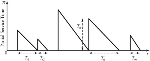

If n and t are large enough, n/t becomes » and & pound ; ⁿ _i=1 T ² _si /n becomes E [ T ² _si ], the second moment of service time. Then, Equation (11.55) can be rewritten as

Equation 11.56

Combining Equations (11.55) and (11.54) forms the Pollaczek-Khinchin (P-K) formula:

Equation 11.57

Clearly, the total queueing time and service time is E [ T _qi ] + E [ T _si ]. By inducing Little's formula, the expected number of packets in the queue, E [ K _qi ], and the expected number of packets in the system, E [ K _i ], we get

Equation 11.58

and

Equation 11.59

These results of the Pollaczek-Khinchin theorem express the behavior of a general distribution of service time modeled as M/G/ 1. For example, if an M/M/ 1 system needs to be expressed by these results, and since service times are exponentially distributed, we have =2/ µ ² , and the Pollaczek-Khinchin formula reduces to

Equation 11.60

Note that the queueing metrics as the expected value of queuing delay obtained in Equation (11.60) is still a function of the system utilization. However, the notion of service rate ¼ has shown up in the equation and is a natural behavior of the non-Markovian service model.

11.5.2. M/D/1 Models

The distribution of service time in a computer network is deterministic. In the asynchronous transfer mode , discussed in Chapter 2, packets are equal sized , and may be so ATM fits well fits in the M/D/ 1 model. When service times are identical for all packets, we have =1/ µ ² . Then:

Equation 11.61

Note that the value of E [ T _qi ] for an M/D/ 1 queue is the lower bound to the corresponding value for an M/G/ 1 model of the same » and ¼ . This is true because the M/D/ 1 case yields the minimum possible value of . It is also worth noting that E [ T _qi ]in an M/M/ 1 queue is twice as much as the one in an M/D/ 1 queue. The reason is that the mean service time is the same in the two cases, and for small s, most of the waiting occurs in the service unit, whereas for large s, most of the waiting occurs within the queue.

11.5.3. Self-Similarity and Batch-Arrival Models

The case of video streaming traffic, which obeys a model in the form of batch arrival , not Poisson, is analyzed in Chapter 18, so our analysis on non-Poisson arrival models is presented there. Here, we give some descriptive and intuitive examples of such models, which give rise to self-similar traffic.

Non-Markovian arrival models , or basically non-Poisson arrival models , have a number of important networking applications. The notion of self-similarity, for example, applies to WAN and LAN traffic. One example of such arrival situations is self-similarity traffic owing to the World Wide Web (WWW). The self-similarity in such traffic can be expressed based on the underlying distributions of WWW document sizes, the effects of caching and user preference in file transfer, and even user think time. Another example of self-similar traffic is video streaming mixed up with regular random traffic backgrounds. In such a case, batches of video packets are generated and are directed into a pool of mixed traffic in the Internet.

Traffic patterns indicate significant burstiness, or variations on a wide range of time scales . Bursty traffic can be described statistically by using self-similarity patterns . In a self-similar process, the distribution of a packet, frame, or object remains unchanged when viewed at varying scales. This type of traffic pattern has observable bursts and thus exhibits long-range dependence. The dependency means that all values at all times are typically correlated with the ones at all future instants. The long-range dependence in network traffic shows that packet loss and delay behavior are different from the ones in traditional network models using Poisson models.