Lesson 3: Editing Data

Editing Cell Content

To edit the content of a cell, press Delete to remove the entire entry. Use any of the following steps to change the content of a cell.

Double-click the cell that contains the data you want to edit.
Press F2 to activate the cursor inside the cell.
Click on the Formula bar where you want to make changes on the cell content.

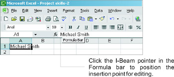
If you want to replace the whole content of the cell, just select it and start typing. The text that you will enter into the cell will overwrite the previous one.

Using Undo and Redo

If you have made a mistake while doing something, the Undo feature of Excel will enable you to recover from the mistake. It also has a Redo feature by which you can reverse the action of the Undo command.

You can find the Undo and Redo button on the Standard toolbar and it has two parts: the button itself and the arrow next to it.

There are some actions you cannot Undo and Redo such as saving, closing, and opening files; as well as maximizing, minimizing, and arranging.

You can do any of the following actions to undo the last action you have made.

Click Undo on the Standard toolbar.
Press Ctrl+Z
Click Edit, choose Undo
Click down arrow beside the Undo button and choose the actions you want to Undo

Note

You can undo up to the last 16 actions.

To cancel Undo immediately, you perform any of the following actions

Click Redo on the Standard toolbar.
Press Ctrl+Y.
Click Edit and choose Redo.
Click down the arrow beside the Redo button and choose the actions you want to redo from the list.

Cut or Move, Copy, and Paste

When you cut or copy an object, graphics or text, it goes to the Windows Clipboard. You can paste any data from the clipboard to any programs you want. There are twenty-four (24) items that you can collect from any programs and store it at the New Office Clipboard wherein you can paste them one at a time or paste them all whenever you need them.

There are many ways to copy, cut, or move and paste cell/s in your worksheet. You can do any of the following:

Select the cell or range of cells, then do either of the following:

To Copy:	To Cut:
Click Edit, choose Copy. Press Ctrl+C. Click the Copy button in the Standard toolbar. Right-click, choose Copy.	Click Edit, choose Cut. Press Ctrl+X Click the Cut button in the Standard toolbar. Right-click, choose Cut.

Select the cell or range of cells where you want the cell/s or object/s to be copied.
To Paste, do any of the following:
- Click Edit, choose Paste.
- Press Ctrl+V.
- Click the Paste button in the Standard toolbar.
- Right-click, choose Paste.

After pasting the content, the Paste option button will appear.

click to expand

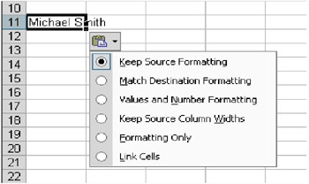
The Paste Options drop-down list displays choices on how your copied text will be formatted. You can turn the Paste Option on or off by doing these steps:

Click Options on the Tools menu, and then click the Edit tab.
Click on the Shadow Paste Options buttons check box.

When you use the Paste command and the desired object or text does not appear, you may do this:

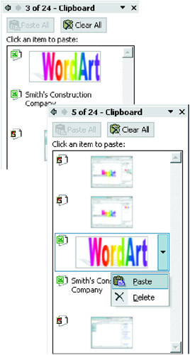
On the Edit menu, click Office Clipboard. The Task pane will display the Office Clipboard.

The Office Clipboard allows you to store up to 24 items of objects. You can paste the objects on the clipboard all at the same time by clicking the Paste All button. You can also delete the content of the clipboard all at once by clicking the Clear All button.

To paste or delete a particular object on the clipboard, follow these steps.

Point to the object that you want to delete or paste. Notice that a drop-down arrow appears.
Click the drop-down arrow and from the available options, click the action you want to perform.

In Excel, the range of cells should be of the same size as the cell range to be copied.

click to expand

Another way to cut, copy, and paste is to use the drag and drop method. To do this, follow the steps below:

Select the cell or range of cells.
Place the mouse pointer to the border of the selected cell/s. The pointer becomes a left-facing white arrow.
Do any of the following:

To Move or Cut:
1. Drag the border to the new location to move the selection.
2. The new location is indicated by a screen tip showing the cell reference before you release the left mouse button.

To Copy:

Hold down the Ctrl key and drag the border to the new location. The white arrow mouse pointer displays a plus sign to indicate that the item is to be copied.

The cell or range of cells you drag can be of different location or even at the Windows desktop.

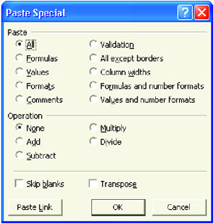
Paste Special

Instead of copying entire cells, you can copy specified contents from the cells, for example, you can copy the format of the cell without copying its content. You can do this by using Paste Special. To do this, follow the steps below:

Select the cells you want to copy.
Click Copy.
Select the upper-left cell of the paste area. Paste Area is the target destination of the selected cells that have been copied or cut.
On the Edit menu, click Paste Special or right-click then choose Paste Special. The Paste Special dialog box appears.
Click OK.

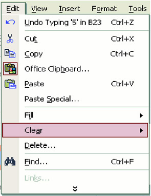
Clear Cell Contents and Formats

While editing, you may erase the content of your cell. You may use the following steps to clear the contents of a cell.

Select the cells, rows or columns you want to clear.
On the Edit menu, point to Clear and choose Contents or press Delete.

The Clear Command has other options that will enable you to clear the formats and comments of a cell. When you choose All it will erase the content, format, and comment of a cell. Formats will only erase the format of the cell and will not erase its content. Choosing Comments will only remove the comments of a cell.

click to expand

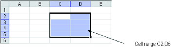
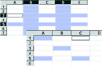
Selecting a Range of Cells

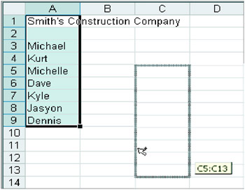
A range is a rectangular block of cells referred to by its upper-left and lower-right diagonal corner cells. For example, the range whose upper-left corner is cell C2 and whose lower-right corner is cell D5 would be referred to as cell range C2:D5. A range can be as small as a single cell or as large as the entire worksheet.

To select a range:

To select a range, click the cell where the selection will start and using the mouse, extend the selection to cover the desired range. Suppose you want to select the range C2:D5.

Click the cell C2.
Hold down the mouse button and drag down to row 5 and across column D to select the range, and then release the mouse button.

Note

You can also use the SHIFT+ARROW keys to select a range of cells.

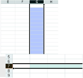
Selecting an Entire Column or Row

Selecting an entire column or row is easy; just click the column or row heading:

Example: To select the entire column G and entire row 7:

Click the column heading (letter) G. This selects the entire column G from G1:G65536.
Click the row heading (number) 7. This selects the entire row 7 from A7:IV7.

Selecting Non-adjacent Cells

To select cells that are apart from each other, follow the steps below.

Select the first cell in the cell range.
Press down the Ctrl key while selecting non-adjacent cells.
Release your hold on the Ctrl key after you are through with your selections.

You can also select non-adjacent rows and columns by selecting the column or row heading then hold down Ctrl key while selecting other headings not adjacent to the first selection.

Inserting and Deleting Selected Cells

If you want to add cell/s to your worksheet, you can select a range of existing cells where you want to insert the new blank cells. In the same way, you can also delete cell/s by selecting the range to be deleted and moving the cells up or to the left.

Selecting non-adjacent cells

click to expand

To insert cell/s, follow these steps:

Move to the cell or range of cells where you want to add cells.
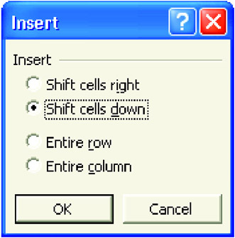
Click Insert and choose Cells. The Insert dialog box will appear.
You can pick any of the following options:
- Shift cells right - moves all the cells that follow the selected cells to the right.
- Shift cells down - moves all the cells that follow the selected cells down.
- Entire row - adds the same numbers of rows. as there are selected rows in your range.
- Entire column - adds the same number of columns, as there are columns in your selected range.
Click OK or press Enter.

Note

You can also use the right-click method to display the Insert dialog box.

When you delete cells, Microsoft Excel removes them from the worksheet and shifts the surrounding cells to fill the space.

To delete cell/s and to move the contents of the other cell/s, follow these steps:

Select the cell or range of cells you want to delete.
From the Edit menu, choose Delete. The Delete dialog box appears.
Choose any of the following:

Shift cells left, Shift cells up, Entire row, and Entire column
Click OK or press Enter.

Note

You can also use the right-click method to display the Delete dialog box.

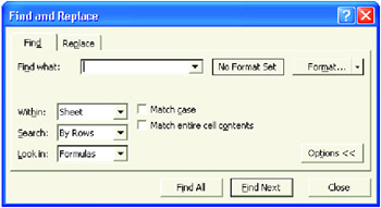
Using Find and Replace

If you do not know the exact location of a text in a worksheet, you can make use of the Find and Replace feature of MS Excel. In the same way, it helps you edit text that you entered incorrectly by using the Replace command.

To find a text, follow these steps:

Activate the Find dialog box:
- Press Ctrl+F.
- From the Edit menu, choose Find. The Find dialog box opens.
Type the text you want to look for in the Find What text box.
Click Find. Notice that the active cell indicator goes to the cell that contains the text you are looking for.
When you have finished, click Close.

To replace a text, follow these steps:

Do any of the following:
- Press Ctrl+H
- From the Edit menu, choose Replace. From the Find and Replace Dialog box, click the Replace tab.
Type the text you want to be replaced in the Find What text box.
In the Replace with box, enter the replacement text with specific formats if necessary. To format it, just click on the Option button then format the text.
Click Replace or Replace All if you want to change that same text in the entire worksheet.
Click Close.

Find and Replace Formats

The Find and Replace feature of Excel not only allows you to find and replace data. It also finds and replaces one type of formatting with another throughout the worksheet. To do this, do the following:

Select a range of cells or press CTRL+HOME to move to the beginning of the worksheet.
Click Edit, then click Replace.
Click the Options button and set options as desired.
Click the arrow on the Find what Format button and select Choose Format From Cell.
Click a cell in the worksheet that has the format you want to change.
Click the Replace with Format button. Select the format you want to use as replacements.
Select Replace or Replace All.
Click Close.

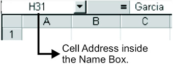
Going to a Specific Cell

The column letter and row number also known as cell reference or cell address identifies a cell. You can move to any cell you want by using the scroll bars and the arrow keys on the keyboard.

If you want to move to a cell that is not currently shown on the screen, you can use any of the following methods:

click to expand

Click the Name box beside the Formula bar.
Type the cell address that you want and press Enter.

Note

You can also move to a cell of another worksheet by typing the sheet reference followed by an exclamation point and cell address (for example: Sheet2!H31).

Another method is by using the Go To command.

From the Edit menu, click Go To or press Ctrl+G. The Go To dialog box appears.
Type the cell address in the Reference text box. The Go To list box shows you the previous location of the active cell indicator.
Press OK.

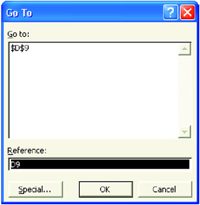
Note

You can also press F5 to open the Go To dialog box.

Whiz Words

Find and Replace	F2
Undo and Redo	Paste Special

Lesson Summary

There are different ways of editing the content of a cell. Before editing the content, you must first select the text you want to edit. You can use the Delete key to overwrite the content of a cell. You can also use the Formula bar, F2, or the double-click method to edit partial content of the cell. And if you want to repeat the last action you take, you can use the Undo and Redo features. You can also remove the format of a cell and its comments. From the Edit menu, click Delete options.

Every time you use Cut and Copy, the Paste command is always needed to complete the task of cutting and copying. There are different ways of performing these tasks. You can use the Menu bar, Shortcut keys, Auto fill, and the click and drag method. Aside from copying entire cells, by using Paste Special you can copy specified contents from the cells, e.g., formats, values, operations, formulas and so on.

You can select adjacent and non-adjacent cells using the mouse or the keyboard. To add cells in a worksheet, you have to select a range of existing cells where you want to insert the new blank cells.

To look for a specific content in a cell, you can use the Find and Replace command. To go to a specific cell, use the Go To command or F5.

Study Help

Directions: Identify the following. Write your answer on the space provided below.

_______________1. The key to be pressed if you want to edit the partial content of a cell.
_______________2. The shortcut for the Undo command.
_______________3. The shortcut for the Redo command.
_______________4. It is identified by its column heading and row number.
_______________5. This feature of MS Excel allows you to locate and replace text.
_______________6. It is a rectangular block of cells referred to by its upper-left and lower-right diagonal corner cells.
_______________7. You store this number of items in the Clipboard.
_______________8. The key to press if you want to go to a specific cell.
_______________9. To select non-adjacent cells, you have to press this while selecting cells.
_______________10. The key to press to activate the Find dialog box.

Activity 1

Open the file Information.xls.
Insert a row before row1
On cell A1, type "Date".
On cell B1, input the current date with this format "March 14, 1998".
Insert a column before A1.
On cell A3, type "1".
Using the auto fill, increment the number by 1.
Edit cell D2 so that the text will appear as Tel. Number.
Undo the last action you made.
Select A1 and B1.
Move the selected cells to cell D1:E1.
Type "My Friends List" cell A1.
Delete the cells that contain the eleventh record.

Delete the last four records.
Save your work.