Chapter 19: The SUMIF, AVERAGEIF, SUMIFS, and AVERAGEIFS Functions
Overview
I’m a sales manager for a makeup company and have summarized for each sales transaction the following information: salesperson, date of sale, units sold (or returned), total price received (or paid out for returns). How can I answer the following questions?
-
What was the total dollar amount of merchandise sold by each salesperson?
-
How many units were returned?
-
What was the total dollar amount of sales in or after 2005?
-
How many units of lip gloss were sold? How much revenue did lip gloss sales bring in?
-
What was the total dollar amount of sales made by someone other than a specific salesperson?
-
What was the average number of units sold in each transaction made by a specific salesperson?
-
What was the total dollar amount of lipstick sold by a specific salesperson?
-
What was the average quantity (in units) of lipstick in each sale made by a specific salesperson?
-
Among transactions involving at least 50 units, what was the average quantity of lipstick in each sale made by a specific salesperson?
-
Among transactions of more than $100, what was the total dollar amount of lipstick sold by a specific salesperson? What about transactions of less than $100?
If you want to sum all the entries in one column (or row) matching criteria that depend on another column (or row), the SUMIF function gets the job done. The syntax of the SUMIF function is SUMIF(range,criterion,[sum range]).
-
Range is the range of cells that you want to evaluate with a criterion.
-
Criterion is a number, date, or expression that determines whether a given cell in the sum range is added.
-
Sum range is the range of cells that are added. If sum range is omitted, it is assumed to be the same as range.
The rules for criteria you can use with the SUMIF function are identical to the rules used for the COUNTIF function. For information about the COUNTIF function, see Chapter 18, “The COUNTIF, COUNTIFS, COUNT, COUNTA, and COUNTBLANK Functions.”
The new AVERAGEIF function has the syntax AVERAGEIF(range,criterion,[average_range]). AVERAGEIF will average the range of cells meeting a criterion.
Microsoft Office Excel 2007 includes three new functions you can use to flag rows that involve multiple criteria: COUNTIFS (discussed in Chapter 18), SUMIFS, and AVERAGEIFS. Other functions that you can use to do calculations involving multiple criteria are discussed in our chapter on database statistical functions (see Chapter 39, “Summarizing Data with Database Statistical Functions”). Array functions (see Chapter 74, “Array Functions and Formulas”) can also be used to handle calculations involving multiple criteria.
The syntax of SUMIFS is SUMIFS(sumrange,range1,criterion1,range2,criterion2,…,rangeN, criterionN). Then SUMIFS will sum up every entry in the sumrange for which criterion1 (based on range1), criterion2 (based on range2),…,criterionN (based on rangeN) are all satisfied. In a similar fashion the new AVERAGEIF function has the syntax AVERAGEIFS(sumrange, range1,criterion1,range2,criterion2,…,rangeN,criterionN). Then AVERAGEIFS will average every entry in the sumrange for which criterion1 (based on range1), criterion2 (based on range2),…, criterionN (based on rangeN) are all satisfied.
-
What was the total dollar amount of merchandise sold by each salesperson?
-
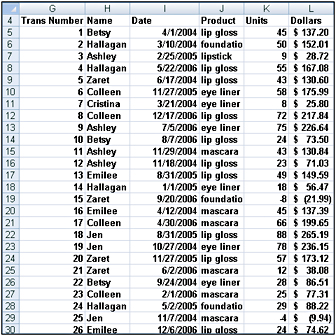
Our work for the problems in this chapter is in the file Makeup2007.xlsx. Figure 19-1 shows a subset of the data.

Figure 19-1: Data we’ll use for SUMIF examples -
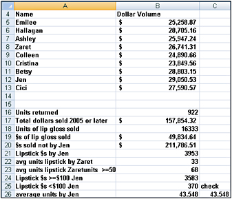
As usual, we begin by labeling the data in columns G through L with the corresponding names in cells G4:L4. For example, the range name Product corresponds to the range J5:J1904. To compute the total amount sold by each salesperson (see Figure 19-2), I simply copy from cell B5 to B6:B13 the formula SUMIF(Name,A5,Dollars). This formula adds up every entry in the Dollars column that contains the name Emilee in the Name column. We find that Emilee sold $25,258.87 worth of makeup. Of course, the formula =SUMIF(Name,"Emilee",Dollars) would yield the same result.

Figure 19-2: Results of SUMIF computations -
How many units were returned?
-
In cell B16, the formula SUMIF(Units,"<0",Units) totals every number less than 0 in the Units column (column K). The result is –922. After inserting a minus sign in front of the SUMIF formula, we see that 922 units were returned. (Recall that when the sum range argument is omitted from a SUMIF function, Excel assumes that sum range equals range. Therefore, the formula –SUMIF(Units,"<0") would also yield 922.)
-
What was the total dollar amount of sales in or after 2005?
-
In cell B17, the formula SUMIF(Date,">=1/1/2005",Dollars) totals every entry in the Dollar column (column L) that contains a date on or after 1/1/2005 in the Date column. We find that $157,854.32 worth of makeup was sold in 2005 or later.
-
How many units of lip gloss were sold? How much revenue did lip gloss sales bring in?
-
In cell B18, the formula SUMIF(Product,"lip gloss",Units) totals every cell in the Units column that contains the text lip gloss in the Product column (column J). You can see that 16,333 units of lip gloss were sold. This is the net sales amount; transactions in which units of lip gloss were returned are counted as negative sales.
-
In a similar fashion, in cell B19 the formula SUMIF(Product,"lip gloss",Dollars) tells us that a net amount of $49,834.64 worth of lip gloss was sold. This calculation counts refunds associated with returns as negative revenue.
-
What was the total dollar amount of sales made by someone other than Jen?
-
In cell B20, the formula SUMIF(Name,"<>Jen",Dollars) sums the dollar amount of all transactions that do not have Jen in the Name column. We find that salespeople other than Jen sold $211,786.51 worth of makeup.
-
What was the average number of units sold in each transaction made by a specific salesperson?
-
This is a job for the AVERAGEIF function. Entering in cell B26 the formula =AVERAGEIF(Name,"Jen",Units) averages every entry in the Units column that contains Jen in the Name column. We find that Jen’s average transaction size was 43.548 units. We verified this in cell C25 with the formula =SUMIF(Name,"Jen",Units)/ COUNTIF(Name,"Jen").
-
What was the total dollar amount of lipstick sold by Jen?
-
This calculation involves two criteria (Name="Jen" and Product="lipstick"). Therefore we compute the desired quantity in cell B21 with the formula =SUMIFS(Dollars,Name, "Jen",Product,"lipstick").
-
We find that the total dollar amount of all transactions in which Jen sold lipstick was $3,953.
-
What was the average quantity (in units) of lipstick in each sale made by Zaret?
-
This calculation requires the AVERAGEIFS function. We compute the desired quantity in cell B22 with the formula =AVERAGEIFS(Units,Name,"Zaret",Product,"lipstick"). We find that for the sales transactions in which Zaret sold lipstick, the average number of units sold was 33.
-
Among transactions involving at least 50 units, what was the average quantity of lipstick in each sale made by Zaret?
-
Again we use AVERAGEIFS, but we add a criterion to ensure units sold in transaction was at least 50. In cell B23, we compute the desired quantity with the formula =AVERAGEIF(Units,Name,"Zaret",Product,"lipstick",Units,">=50"). We find that in all transactions in which Zaret sold at least 50 units of lipstick, the average transaction size was 68 units.
-
Among transactions of more than $100, what was the total dollar amount of lipstick sold by Jen? What about transactions of less than $100?
-
Because our criteria is Name=Jen, Product=lipstick, and some statement about the dollar size of each order, we need to use the SUMIFS function. In cell B24 we compute the total amount in transactions in which Jen sold lipstick and the dollar amount was at least $100 with the formula =SUMIFS(Dollars,Name,"Jen",Product,"lipstick",Dollars">=100"). We find that Jen sold $3,583 worth of lipstick in such transactions. In lipstick transactions involving less than $100, we find in cell B25 (formula is =SUMIFS(Dollars,Name, "Jen",Product,"lipstick",Dollars,"<100") the answer is $370. Note that $370+$3,583 equals the total revenue Jen generated from lipstick sales (computed in cell B21).
EAN: 2147483647
Pages: 200