Chapter 70: Estimating a Demand Curve

Overview

• What do I need to know to price a product?

• What is the meaning of elasticity of demand?

• Is there any easy way to estimate a demand curve?

• What does a demand curve tell us about a customer’s willingness to pay for our product?

Every business must determine a price for each of its products. Pricing a product properly is difficult. In Chapter 71, “Pricing Products by Using Tie-Ins,” and Chapter 72, “Pricing Products by Using Subjectively Determined Demand,” I’ll describe some simple models that might aid you in pricing a product to maximize profitability. For further insights into pricing, refer to the excellent book Power Pricing, by Robert J. Dolan and Hermann Simon (Free Press, 1996).

• What do I need to know to price a product?

• Let’s consider a product such as a candy bar. In order to determine a profit-maximizing price, we need to know two things:

  • The variable cost of producing each unit of the product (we’ll call this UC).

  • The product’s demand curve. Simply put, a demand curve tells us the number of units of our product a customer will demand at each price. In short, if we charge a price of $p per unit, the demand curve gives us a number D(p), which equals the number of units of our product that will be demanded at price $p. Of course, a firm’s demand curve is constantly changing and often depends on factors beyond the firm’s control (such as the state of the economy and a competitor’s price).

• After we know UC and the demand curve, the profit corresponding to a price of $p is simply (p–UC)*D(p). After we have an equation for D(p), which gives the quantity of the product demanded for each price, we can use the Microsoft Office Excel Solver feature to find the profit-maximizing price, which we’ll do in Chapters 71 and 72.

• What is the meaning of elasticity of demand?

• Given a demand curve, the price elasticity for demand is the percentage decrease in demand resulting from a 1 percent increase in price. When elasticity is larger than 1 percent, demand is price elastic. When demand is price elastic, a price cut will increase revenue. When elasticity is less than 1 percent, demand is price inelastic. When demand is price inelastic, a price cut will decrease revenue. Here are some observed estimates of elasticities:

  • Salt, 0.1 (very inelastic)

  • Coffee, 0.25 (inelastic)

  • Legal fees, 0.4 (inelastic)

  • TV sets, 1.2 (slightly elastic)

  • Restaurant meals, 2.3 (elastic)

  • Foreign travel, 4.0 (very elastic)

• A 1 percent decrease in the cost of foreign travel, for example, will result in a 4 percent increase in demand for foreign travel.

• Is there any easy way to estimate a demand curve?

• Using q to represent the quantity demanded of a product, the two most commonly used forms for estimating demand curves are as follows:

• Linear demand curve.   In this case, demand follows a straight line relationship of the form q=a–bp. For example, q=10–p is a linear demand curve. (Here a and b can be determined by using a method that I’ll describe later in the chapter.) When the demand curve is linear, the elasticity is constantly changing.

• Power Demand Curve.   In this situation, the demand curve is described by a power curve of the form q=ap^b, b<0. (See Chapter 45, “The Power Curve,” for a discussion of the power curve.) Again, a and b can be determined by the method I’ll describe later in the chapter. The equation q=100p^-2 is an example of a power demand curve. If demand follows a power curve, for any price, the elasticity equals –b. Thus, for the demand curve q=100p^-2, the price elasticity of demand always equals 2.

• Suppose that a product’s demand curve follows a linear or power demand curve. Given the current price and demand for a product and the product’s price elasticity of demand, determining the product’s demand curve is a simple matter. Here are two examples.

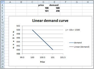
• A product is currently selling for $100 and demand equals 500 units. The product’s price elasticity for demand is 2. Assuming the demand curve is linear, we want to determine the equation of the demand curve. Our solution is in the file Linearfit.xlsx, which is shown in Figure 70-1.

  
  Figure 70-1: Fitting a linear demand curve

• Given two points, we know that there is a unique straight line that passes through those two points. We actually know two points on our demand curve. One point is p=100 and q=500. Because elasticity of demand equals 2, a 1 percent increase in price will result in a 2 percent decrease in demand. Thus, if p=101 (a 1 percent increase), demand will drop by 2 percent of 500 (10 units), or 490. Thus p=101 and q=90 is a second point on our demand curve. We can now use the Excel trendline to find the straight line that passes through the points (100,500) and (101,490).

• We begin by entering these points in our worksheet in the cell range D5:E6, as shown in Figure 70-1. Then we select the range D4:E6 and on the Ribbon, in the Charts group choose Scatter, Scatter With Straight Lines. After selecting this option for a Scatter chart we see the graph has a positive slope. This would imply that higher prices lead to higher demand, which cannot be correct. The problem is that with only two data points, Excel assumes that the data points we want to graph are in separate columns, not separate rows. To ensure Excel understands that the individual points are in separate rows, simply click inside the graph and on the Ribbon, click the Design tab in the Chart Tools section. Click Switch Row/Column in the Data section of the Design tab. Note that by clicking the Select Data button, you can change the source data that generates your chart. Now we right-click one of the points, click Add Trendline, and then click the Linear and the Display Equation On Chart options. After clicking OK in the Add Trendline dialog box, you will see the straight line plot, complete with the equation shown in Figure 70-1. Because x is price and y is demand, the equation for our demand curve is q=1500–10p. This equation means that each $1 increase in price costs us 10 units of demand. Of course, demand cannot be linear for all values of p because for large values of p, a linear demand curve will yield negative demand. For prices near the current price, however, the linear demand curve is usually a good approximation to the product’s true demand curve.

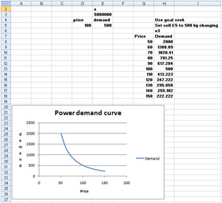
• As a second example, let’s again assume that a product is currently selling for $100 and demand equals 500 units. The product’s price elasticity for demand is 2. Now let’s fit a power demand curve to this information. See the file Powerfit.xlsx, shown in Figure 70-2.

  
  Figure 70-2: Power demand curve

• In cell E3, we enter a trial value for a. Then, in cell D5, we enter the current price of $100. Because elasticity of demand equals 2, we know that the demand curve has the form q=ap^-2, where a is unknown. In cell E5, we enter the demand for a price of $100, corresponding to the value of a in cell E3, with the formula a*D5^-2. Now we use the Goal Seek command (for details, see Chapter 16, “The Goal Seek Command”) to determine the value of a that makes our demand for price $100 equal to 500 units. I simply set cell E5 to the value of 500 by changing cell E3. I find that a value for a of 5 million yields a demand of 500 at a price of $100. Thus, our demand curve (graphed in Figure 70-2) is given by q=5,000,000p^-2. For any price, the price elasticity of demand on this demand curve equals 2.

• What does a demand curve tell us about a customer’s willingness to pay for our product?

• Let’s suppose we are trying to sell a software program to a Fortune 500 company. Let q equal the number of copies of the program the company demands, and let p equal the price charged for the software. Suppose we have estimated that the demand curve for software is given by q=400–p. Clearly, our customer is willing to pay less for each additional unit of our software program. Locked inside this demand curve is information about how much the company is willing to pay for each unit of our program. This information is crucial for maximizing profitability of sales.

• Let’s rewrite our demand curve as p=400–q. Thus, when q=1, p=$399, and so on. Now let’s try and figure out the value our customer attaches to each of the first two units of our program. Assuming that our customer is rational, the customer will buy a unit if and only if the value of the unit exceeds our price. At a price of $400, demand equals 0, so the first unit cannot be worth $400. At a price of $399, however, demand equals 1 unit. Therefore, the first unit must be worth somewhere between $399 and $400. Similarly, at a price of $399, the customer does not purchase the second unit. At a price of $398, however, the customer is purchasing two units, so the customer does purchase the second unit. Therefore, the customer values the second unit somewhere between $399 and $398.

• It can be shown that the best approximation to the value of the ith unit purchased by the customer is the price that makes demand equal to i–0.5. For example, by setting q equal to 0.5, we find that the value of the first unit is 400–0.5=$399.50. Similarly, by setting q=1.5, we find that the value of the second unit is 400–1.5=$398.50.