Lesson 4: Managing Performance
Managing performance is an ongoing task that includes optimizing the design of your data warehouse as well as monitoring and analysis. In this lesson, you will learn how to design and optimize your data warehouse databases. You will learn more about using multiple partitions in an OLAP Services database when you are running SQL Server OLAP Services Enterprise Edition. You will learn how to use the Usage-Based Optimization wizard and the Usage Analysis wizard.
After this lesson, you will be able to:
- Describe optimization strategies for a data warehouse
- Describe optimization strategies for cubes
- Create cube partitions
- Optimize performance by determining appropriate levels of aggregations, indexing, and storage methods
Estimated lesson time: 120 minutes
Optimizing Data Warehouse Performance
You can apply several important tuning steps to your data warehouse to optimize performance.
Use Effective Indexing
Data in your data warehouse or data mart should be indexed properly to minimize the time required to extract the data from the relational system while building cubes. You should
- Create an index on all primary key and foreign key columns to provide the most efficient joins between tables.
- Create a composite index on fact table keys.
- Keep statistics current by taking advantage of automatic statistics generation or other available means in SQL Server databases. Doing so allows the SQL Server optimizer to make the best decisions about when to use indexes rather than table scans.
- Use the Index Tuning wizard in SQL Server to assist you in determining appropriate indexes.
TIP
Create a clustered index on each dimension table on a column or group of columns that are searched frequently in ranges or are accessed in sorted order. For a large fact table, you should not create a clustered index because clustered indexes are to expensive to maintain. The organization of rows is maintained when new data is added to the fact table because typically the existing data is not updated in a warehouse
Denormalize the Schema to Reduce the Number of Joins
In your data warehouse or data mart, you should denormalize the schema to reduce the number of joins required when the data is queried. Typically, you will use a star schema to accomplish this reduction.
Optimizing Cube Design
Optimizing cube performance starts with solid cube design. To ensure that your cubes are designed most efficiently, consider the following factors.
Reduce Cube Complexity
You should strive to reduce unnecessary complexity in your cubes by analyzing exactly what information is needed. You should use the minimum number of dimensions, levels, or members necessary to accomplish the desired task.
Optimize Schema in Cube Editor
Removing unneeded dimensions, levels, and members from cubes can greatly increase the performance of processing and querying. Additionally, you can optimize the cube schema by removing unnecessary joins in the data warehouse tables.
When optimizing your cube, you can use the Optimize Schema option on the Tools menu in the Cube Editor to help identify potential deficiencies in your cube design. In general, if you are using a single data warehouse as a source, you should ensure that it is optimized first. If you are using more than one data source, you may need to optimize the schema in the cube.
Creating Partitions
Using partitions can significantly improve query performance, particularly on multiprocessor systems or when you have partitioned a cube across two or more servers. When you use multiple partitions on multiprocessor systems, the query parser is able to divide the workload more efficiently among the processors to improve performance.
Each partition uses two operating system threads: one to read data from the data warehouse and one to load data into the cube and create aggregations and indexes. By using multiple partitions, OLAP Services can perform processing simultaneously on different parts of the cube, provided there are sufficient hardware resources available and the OLAP Server has been configured properly.
Using Cube Partitions
When you create a cube, at least one partition is automatically created to store cube data. You can use the Partition wizard to create partitions and store a cube across many partitions. From the users perspective, partitions have no effect on the cube. Figure 14.7 shows how you can partition the Sales cube based on yearly data.
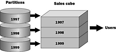
Figure 14.7 Partitioning the Sales cube based on yearly data
Reasons to Create Partitions
Creating additional partitions allows you to
- Increase scalability over systems using a single partition per cube
- Segment parts of a cube to store different partitions of data
- Specify a different storage format for each partition
- Set individual optimization to help manage the size of large cubes
- Enhance query performance
TIP
To create partitions that will be candidates for later merging, you can select the storage mode and copy aggregations from another partition when you create the partition.
Scenario Example
An organization determines that the best way to store its data is in one cube, partitioned by age, because most queries are performed using the time dimension. In this scenario, the last partition is incrementally updated nightly, and as long as the history partition doesn t change, the cube does not have to be reprocessed.
- Pre-1995 data is stored in a ROLAP partition with few aggregations, because it is queried infrequently.
- Data for 1995 is stored in a HOLAP partition.
- Data for 1996 1998 is stored in individual MOLAP partitions with more aggregations.
- Monthly 1999 data is stored in MOLAP partitions with an identical high level of aggregations. At the end of a quarter, the months in that quarter are merged into a quarterly partition; quarterly partitions will be eventually merged into the partition for the year.
Allocating Data to Partitions
You should consider additional configuration settings when optimizing your configurations. In this section we take a closer look at aligning fact tables and partitions for optimal performance and maintainability. Different Fact Table for a Partition
As you see in the top of Figure 14.8, you can define a fact table for a partition that is different from that defined for the primary partition of the cube. This type of partition is useful when you want to store different types of data, such as different product lines, on separate partitions.
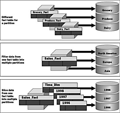
Figure 14.8 Allocating data to partitions
When creating this type of partition, you must ensure that the fact table structure is the same as the primary fact table structure. For example, you may store different products in different fact tables, but all the tables must have the same structure. You could place these different fact tables on different partitions.
Filter Data from One Fact Table into Multiple Partitions
In the second example of Figure 14.8, you see that it is possible to break up a single cube over multiple partitions. This is similar to data slicing, but it has greater flexibility because the division criteria do not have to be along dimension lines. Extra care must be taken to ensure that there is no duplicate data in the partitions.
Slice Data from One Fact Table into Multiple Partitions
In the final example of Figure 14.8, it shows that you can also slice across dimensions and store each dimensional data slice in a separate partition. This type of partition is useful for queries that access only a certain subset of a dimension, such as the current year. For example, if you have a multiple-year dimension, you may put individual years on separate partitions. This is a slice of the Time dimension.
By determining the cost of adding cubes compared with the query performance, you should carefully analyze how the data is sliced or whether to slice data at all.
NOTE
Only SQL Server OLAP Services Enterprise Edition running on Windows NT Enterprise Edition supports the partitioning feature of OLAP Services.
Merging Partitions
Although it is not typically desirable to merge partitions, Microsoft has provided the functionality necessary to perform this task. It is important to plan your partitions carefully to get optimal performance and to avoid unnecessary merges. As you will see in this section, merging is a complex process that can cause errors in your data if it is not performed correctly.
Determining Which Partitions to Merge
When determining which partitions to merge, you must ensure that all partitions
- Have the same structure
- Are saved in the same storage format (ROLAP, HOLAP, or MOLAP)
- Contain identical aggregation design
OLAP Services will not allow you to merge partitions that do not meet these requirements.
Merging Sliced Data
If you merge partitions created by slicing, the merged partition can contain incorrect data after it is processed.
For example, your data is sliced by regions (Region 1, Region 2, and Region 3), all of which are part of a territory (Territory 1). Each region is stored in a different partition. If you merge the Region 2 and Region 3 partitions, when you process the data in the merged partition, the content of the merged partition will default to the parent of the regions, which is Territory 1. After processing the cube, the second partition will now include the data from Region 1, Region 2, and Region 3. Region 3 would therefore be duplicated. To avoid duplication, you need to define a filter on the merged partition that limits its contents to Region 2 and Region 3.
Merging Partitions That Use Different Fact Tables
If two partitions use different fact tables, the merged partition will use only the fact table of the target partition; you must manually merge the fact table of the source partition into the fact table of the target partition. After you merge partitions with different fact tables, it is important to process the cube. Failure to do so can show the user accurate aggregations but incorrect base data.
Managing Partitions
Whether you create or merge partitions, you must manage these activities to ensure that the partitions of a cube always contain the correct data.
Ensuring Data Consistency
Data consistency in the cube is the primary concern when creating and merging partitions. Inconsistent data produces incorrect summaries and presents erroneous data to users.
For example, if a sales transaction for Product n is duplicated in the fact tables for two partitions, summaries of Product n sales can include a double accounting of the duplicated transaction.
To ensure data consistency, it is important to create appropriate filters for your partitions.
Defining Filters
When you partition cube data, you can explicitly define a filter in the definition of a partition to minimize unexpected effects on data that changes to the underlying data warehouse data can cause. Explicitly defined partition filters have different effects depending on the specific storage structure of the partition. These differences are shown in the following table.
| Storage | Filter Effect |
|---|---|
| MOLAP | Specifies which data is read from the data warehouse to create aggregations when the cube is processed. New data is not available until the cube is reprocessed. |
| ROLAP and HOLAP | Specifies which data from the data warehouse can be accessed by queries. New data is available to queries immediately, which can cause data inconsistencies. For this reason, it is often important to use a filter to explicitly exclude new data. |

Optional Exercise: Creating a Cube with Multiple Partitions
In this exercise, you will use OLAP Manager to create a new database in OLAP Services. You will then create multiple partitions for the Sales cube.
You must be using OLAP Services Enterprise Edition in order to complete this exercise.
In this procedure, you will use OLAP Manager to create a new database called Northwind_Partition and add a data source for the database.
- In OLAP Manager, expand OLAP Servers, and then expand your server.
- Right-click your server, and then click New Database.
- Type Northwind_Partition for the name of the database, and then click OK.
- In the console tree, expand the Northwind_Partition database, and then expand the Library folder.
- Right-click Data Sources, and then click New Data Source.
- Use the following information to define the data source.
- Click Test Connection to verify the connection, then click OK to close the Data Link Properties dialog box.
| Option | Value |
|---|---|
| Provider | Microsoft OLE DB Provider for SQL Server |
| Server name | Your server name |
| Log on to the server | Use Windows NT Integrated Security |
| Database | Northwind_Mart |
In this procedure, you will build the Time dimension.
- In the console tree, open the Library folder, right-click the Shared Dimensions folders, point to New Dimension, and then click Wizard.
- Use the information in the following table to build the Time dimension.
- Click Finish to complete the wizard and to go to the Dimension Editor.
| Option | Value |
|---|---|
| Create a new dimension from | A single-dimension table |
| Dimension table | Time_Dim |
| Dimension type | Time dimension |
| Date_column | TheDate |
| Time levels | Year, Quarter, Month, Day |
| Dimension name | Time |
In this procedure, you will build the Product dimension.
- On the Dimension Editor toolbar, click File, point to New Dimension, and then click Wizard.
- Use the information in the following table to build the Product dimension.
- Click Finish to complete the wizard and to go to the Dimension Editor.
| Option | Value |
|---|---|
| Create a new dimension from | A single-dimension table |
| Dimension table | Product_Dim |
| Dimension levels | CategoryName and ProductName columns, in that order |
| Dimension name | Product |
In this procedure, you will build the Customer dimension.
- On the Dimension Editor menu, click File, point to New Dimension, and then click Wizard.
- Use the information in the following table to build the Customer dimension.
| Option | Value |
|---|---|
| Create a new dimension from | A single-dimension table |
| Dimension table | Customer_Dim |
| Dimension levels | Country, Region, City, and CompanyName columns, in that order |
| Dimension name | Customer |
NOTE
When defining some levels, you may receive warning messages that the number of children is less than the number of parents. In the cube, this message is expected when defining the Region level in the Customer dimension. The Region column stores the state or province for each country. Some countries do not have Region attributes. Click Yes when this message occurs.
- Click Finish to complete the wizard and to go to the Dimension Editor.
In this procedure, you will build the Shipper dimension.
- On the Dimension Editor menu, click File, point to New Dimension, and then click Wizard.
- Use the information in the following table to build the Shipper dimension.
- Click Finish to complete the wizard and to go to the Dimension Editor.
- On the File menu, click Exit to close the Dimension Editor.
| Option | Value |
|---|---|
| Create a new dimension from | A single-dimension table |
| Dimension table | Shipper_Dim |
| Dimension levels | ShipperName |
| Dimension name | Shipper |
In this procedure, you will use the Cube wizard to define the Sales cube.
- In the console tree, expand the Northwind_Partition database.
- Right-click the Cubes folder, point to New Cube, and then click Wizard.
- Use the information in the following table to define the cube.
- Click Finish to close the wizard and go to the Cube Editor.
- Close the Cube Editor. Do not process the cube or design aggregations at this time.
| Option | Value |
|---|---|
| Select a fact table | Sales_Fact |
| Select numeric columns that define your measures | Line Item Total, Line Item Quantity, and Line Item Discount columns, in that order |
| Select the dimensions for your cube | Time, Product, Customer, and Shipper |
| Cube name | Sales |
In this procedure, you will use the Partition wizard to partition the Sales cube by using the data slice method.
- In the console tree, expand your server, expand the Northwind_Partition database, and then expand Cubes.
- Expand Sales, right-click Partitions, and then click New Partition.
- Use the information in the following table to partition the Sales cube. Accept the defaults for any options that are not listed.
- Click Finish to go to the Storage Design wizard.
- Use the information in the following table to design storage and aggregations.
- Click Finish.
- Repeat steps 2 through 6 to create partitions for 1997 and 1998. Use 1997 and 1998 as the Time dimension members and name these partitions "Year 1997" and "Year 1998," respectively. Use the same storage options and aggregations as you used for the partition for 1996.
- In the console tree, expand Partitions for the Sales cube, right-click the Sales partition, and choose Delete. Your Sales cube will now contain only the partitions data sliced by year.
| Option | Value |
|---|---|
| Data source | Northwind_Mart |
| Fact table | Sales_Fact |
| Select the data slice | Time dimension, member 1996 |
| Partition name | Year 1996 |
| Design aggregations for your partition now | Selected |
| Option | Value |
|---|---|
| Data storage type | MOLAP |
| Aggregation options | Performance gain reaches 50% |
| Create aggregations | Click Start Notice the Performance vs. Size graph and the number of aggregations designed for you. |
| Save, but don't process now | Selected |
In this procedure, you will process the Sales cube.
- Expand the Northwind_Partition database, expand Cubes, right-click the Sales cube, and then click Process. Click OK to process the cube. When processing is complete, click Close to close the Process dialog box.
- Right-click the Sales cube, and then choose Browse Data.
- In the Cube Browser, select different years from the Time dimension at the top of the screen to view data for a particular year. Notice that the partitions are transparent to users querying the data.
Optimizing Based on Usage
To ensure that you have processed the most efficient and frequently used aggregations, you should audit the queries that have been submitted by users. SQL Server OLAP Services provides the Usage Analysis wizard and the Usage-Based Optimization wizard to help you to optimize your cubes based on usage.
TIP
SQL Server provides extensive monitoring capability that is integrated with the Windows NT Performance Monitor. You should perform standard performance monitoring and analysis of SQL Server in addition to using the OLAP Services analysis tools covered in this lesson.
Set Aggregation Levels Based on Query History
Aggregations improve query speed but come with the cost of increased disk storage space and cube processing time. By reviewing the queries that users submit, you can determine which aggregations can answer the majority of queries and can eliminate unnecessary ones.
Usage-based aggregations can be used to set aggregation levels automatically based on actual query history. This can be particularly useful when the same types of queries are used repeatedly. Run the Usage-Based Optimization wizard to create aggregations based on actual query history.
NOTE
As we discussed in Lesson 4 of Chapter 9, "Managing Cubes Using Storage Types and Partitions," the storage method that you choose also affects the performance of OLAP Services. Review the table in Chapter 9 that compares MOLAP, ROLAP, and HOLAP.
Exercise 1: Using the Usage-Based Optimization Wizard
In this exercise, you will use the Usage-Based Optimization wizard to process the Sales cube in the Northwind_DSS database based on the queries that you have run on the Sales cube.
- In OLAP Manager, expand Northwind_DSS and right-click the Sales cube, then click Usage-Based Optimization.
- The Usage-Based Optimization wizard dialog box opens. Click the Next button.
- Review the filter options for the queries that you want to optimize. Check the Queries that took longer than check box. Leave the time as 0 seconds so those queries that took at least 1 second to run will be optimized.
- Click the Next button.
- The results table shows the queries that meet the selected filter options. These are the queries that will be used to perform the optimization. Click the Next button.
- Click the Replace the existing aggregations option, and then click the Next button.
- Click the ROLAP option, and then click the Next button.
- Click the Performance gain reaches option, and then type in 80 in the % text box.
- Click the Start button and watch the performance optimization graph and the number of aggregations that are designed.
- Click the Next button.
- Click the Finish button to process the Sales cube with the newly designed aggregations.
- The Process dialog box shows the progress of the cube processing. When the processing completes, click the Close button.
Analyze Cube Usage
You can run the Usage Analysis wizard to see reports that show information about the queries that have been submitted. Reports are in either a tabular or a histogram graph format. The following reports are available:
- Query Run-Time Table
- Query Frequency Table
- Active User Table
- Query Response Graph
- Query by Hour Graph
- Query by Date Graph
A table that shows the length of time it takes each query to run. The queries are ordered from the longest to the shortest runtime.
A table that shows how frequently each query is run. The queries are ordered from the most frequently to the least frequently run query.
A table that shows the number of queries that have been run by each user. The table is ordered from the most active to the least active user.
A histogram that graphs query response times in ranges from fewer than 5 seconds to more than 60 seconds.
A histogram that graphs the number of queries that run during each hour of the day.
A histogram that graphs the number of queries that run grouped by date.
You can filter the reports on the following criteria:
- Queries that run during a selected calendar week
- Queries that take longer than a specified time to run
- Queries that have been run more than a specified number of times
- Queries that have been run by selected users
Review Query Log Sample Frequency
The Usage-Based Optimization wizard and Usage Analysis wizard rely on query history logging. By default, every tenth query received by the OLAP Server is logged. You can set the logging frequency on the Query Log tab in the Server Properties dialog box.
Exercise 2: Using the Usage Analysis Wizard
In this exercise, you will view Usage Analysis wizard reports for the Northwind_DSS database.
- In OLAP Manager, expand Northwind_DSS and right-click the Sales cube, then click Usage Analysis.
- The Usage Analysis wizard dialog box opens.
- Select one of the reports, and click the Next button.
- Review the filter options for the report, and then click the Next button.
- The report is displayed. Note that you can delete the usage history by clicking the Delete Records button. Click the Finish button to close the wizard and return to OLAP Manager, or you can click the Back button twice to select a different report.
- Repeat steps 2 through 5 for each of the reports.
Lesson Summary
Effective use of indexes and optimal design of your SQL Server databases and OLAP Services cubes are essential for gaining the best performance from your data warehouse. Using multiple partitions provides scalability, increased manageability, and increased performance if you are running SQL Server OLAP Services Enterprise Edition. The Usage-Based Optimization wizard and the Usage Analysis wizard are useful tools for tuning your OLAP Services cubes based on actual user query patterns.
EAN: 2147483647
Pages: 114