10.4 Model Construction
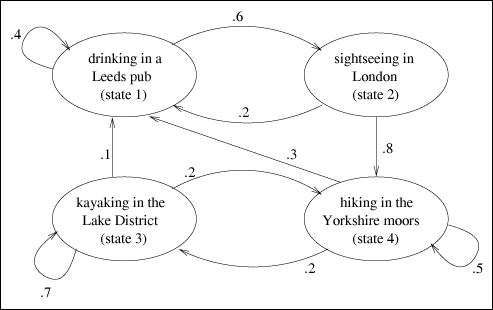
| As illustrated in Fig. 10.1, the first step when modeling a system is to construct the model. This involves enumerating the state space, identifying the state transitions, and parameterizing the model. These tasks are illustrated on both of the motivating examples. Random Walk Through England: Model Construction In order to construct the model, the first task is to enumerate all the possible states in which the system might find itself. This is the system's "state space." In this example, there are four possible states in which the mother may find the lad:
This state space is mutually exclusive and collectively exhaustive. This means that it is not possible to be in more than one state at a time (i.e., mutually exclusive) and that it is not possible to be in any state other than in one of the identified states (i.e., collectively exhaustive). The second task is to identify the state transitions. These are the "single step" transitions. That is, if the system (i.e., the lad) is in one state, identify those possible states that the system may find itself during the immediately following time step (i.e., the next day). In the current example, the following are the possible state transitions.
The third task is to parameterize the model. This involves assigning weights to each of the state transitions. These weights indicate the flow rates (i.e., how likely it is to transition) from one state directly to another. In the example, these weights are given as probabilities.
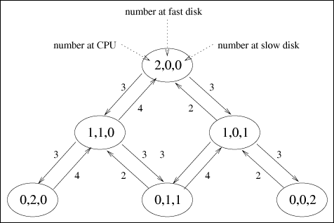
The complete model can be represented by the Markov state diagram shown in Fig. 10.4. Figure 10.4. Markov model of the England example. Database Server Support: Model Construction (Refer to Fig. 10.3.) As in the England example (and in all Markov models), the first task is to enumerate all possible system states. In the England example, it was very straightforward. There was one user (i.e., the lad) who could be in one of four states. In this example, things are slightly more complex since there are two users, each of which could be at any of the three devices (i.e., CPU, fast disk, slow disk). However, by adopting the notation (X,Y,Z), where X denotes the number of users currently at the CPU, Y denotes the number of users at the fast disk, and Z denotes the number of users at the slow disk, the six possible states are:
Often, a crucial part of the modeling process is to come up with good notation to describe each state. In this example, the tuple (X,Y,Z) is selected. Alternatively, the notation (A,B) could have been used, where A denotes the location of the first user (i.e., either at the CPU, fast disk (FD), or slow disk (SD)), and B denotes the location of the other user. This would lead to the following nine states: (CPU,CPU), (CPU,FD), (CPU,SD), (FD,CPU), (FD,FD), (FD,SD), (SD,CPU), (SD,FD), and (SD,SD). However, since both users are (statistically) identical, states such as (CPU,FD) and (FD,CPU) are equivalent and can be combined. Thus, although the resulting performance measures would be identical, the latter notation leads to a more complex model. Similarly, consider the notation (I,J;K,L;M,N), where I denotes the user ID number (i.e., either -, 1, or 2) of the job, if any, which is waiting in the queue to use the CPU, and where J denotes the user ID number (i.e., either -, 1, or 2) of the job, if any, which is currently using the CPU. (Similarly, K and L denote the user ID number of any user waiting for and using the fast disk, respectively. M and N, likewise, represent the state at the slow disk.) This notation leads to 12 feasible states: (2,1; , ; , ), (1,2; , ; , ), ( ,1; ,2; , ), ( ,2; ,1; , ), ( ,1; , ; ,2), ( ,2; , ; ,1), ( , ;2,1; , ), ( , ;1,2; , ), ( , ; ,1; ,2), ( , ; ,2; ,1), ( , ; , ;2,1), and ( , ; , ;1,2). This notation not only distinguishes between user 1 and user 2 as in the previous notation, but also distinguishes between which user is getting service at a device and which user is waiting for service, if they are both at the same device. These latter two notations would be necessary in a multi-class model (see Chapter 12) where the characteristics of the users and the queues are different. However, such notations only add complexity here. The point of note is that the choice of notation to represent each state is important. The second task is to identify the state transitions. These follow straightforwardly.
The third model construction task, parameterization, involves assigning weights to each of the state transitions. In the England example, these weights are given as simple transition probabilities. In the database server example, these are given as "flow rates," which is a generalization of transition probabilities. For example, suppose the system is in state (2,0,0) where both users are at the CPU. In this state, the CPU is actively working, satisfying user requests at a rate of 6 transactions per minute (since it takes an average of 10 seconds to satisfy one typical user's CPU demand). Of the 6 transactions per minute that the CPU can fulfill, half of these transactions next visit the fast disk (i.e., to state (1,1,0)) and half next visit the slow disk (i.e., to state (1,0,1)). Therefore, the weight assigned to the (2,0,0) As another example, consider state (1,1,0) where one user is executing at the CPU and the other user is using the fast disk. As before, the user at the CPU leaves at rate 6, half the time going to the fast disk and half the time going to the slow disk. Thus, the weight assigned to the (1,1,0) Using similar reasoning, it is relatively straightforward to parameterize all possible state transitions. The complete model can be represented by the Markov state diagram shown in Fig. 10.5. Figure 10.5. Markov Model of the database server example. |
EAN: 2147483647
Pages: 166

 (1,1,0) transition is 3 and the weight assigned to the (2,0,0)
  (0,2,0) transition is 3 and the weight assigned to the (1,1,0)