Excel Macros

This section takes you through a few useful macros that you can use when working with Excel worksheets.

Assigning Shortcut Keys to Excel Macros

Before getting to some specific procedures, let's take a brief side trip to discuss assigning shortcut keys to Excel macros. The easiest way to assign a shortcut key to an existing macro (or change a macro's current shortcut key) is to follow these steps:

1.	Select Tools, Macro, Macros (or press Alt+F8) to display the Macro dialog box.
2.	Select the macro you want to work with.
3.	Click Options to display the Macro Options dialog box shown in Figure 12.4. Figure 12.4. Use the Macro Options dialog box to assign a shortcut key to a macro.
4.	In the Shortcut Key Ctrl+ text box, type the letter you want to use with Ctrl for the key combination. For example, if you type e, you can run the macro by pressing Ctrl+E. Excel Shortcuts Are Case Sensitive Excel shortcut keys are case sensitive, meaning you can create separate shortcuts with uppercase and lowercase letters. For example, if you type e into the Ctrl+ text box, you would have to press Ctrl+E to run the macro. However, if you type E into the Ctrl+ text box, you would have to press Ctrl+Shift+E to run the macro.
5.	Click OK to return to the Macro dialog box.
6.	Click Cancel.

Avoid Shortcut Key Conflicts

Make sure you don't specify a shortcut key that conflicts with Excel's built-in shortcuts (such as Ctrl+B for Bold or Ctrl+C for Copy). If you use a key that clashes with an Excel shortcut, Excel will override its own shortcut and run your macro instead (provided that the workbook containing the macro is open).

There are only five letters not assigned to Excel commands that you can use with your macros: e, j, m, q, and t. You can get extra shortcut keys by using uppercase letters. For example, Excel differentiates between Ctrl+b and Ctrl+B (or, more explicitly, Ctrl+Shift+b). Note, however, that Excel uses four built-in Ctrl+Shift shortcuts: A, F, O, P.

There are two major drawbacks to assigning Ctrl+key combinations to your Excel macros:

• Excel uses some Ctrl+key combinations for its own use (such as Ctrl+O for Open and Ctrl+G for Go To), which limits the key combinations that you can use.

• It doesn't help if you would like your procedures to respond to "meaningful" keys such as Delete and Esc.

To remedy these problems, use the Application object's OnKey method to run a procedure when the user presses a specific key or key combination:

 Application.OnKey(Key, Procedure) 

Key	The key or key combination that runs the procedure. For letters, numbers, or punctuation marks, enclose the character in quotes (for example, "a"). For other keys, see Table 12.1.
Procedure	The name (entered as text) of the procedure to run when the user presses a key. If you enter the null string ("") for Procedure, a key is disabled. If you omit Procedure, Excel resets the key to its normal state.

Table 12.1. Key Strings to Use with the OnKey Method

Key	What to Use
Backspace	"{BACKSPACE}" or "{BS}"
Break	"{BREAK}"
Caps Lock	"{CAPSLOCK}"
Delete	"{DELETE}" or "{DEL}"
Down arrow	"{DOWN}"
End	"{END}"
Enter (keypad)	"{ENTER}"
Enter	"~" (tilde)
Esc	"{ESCAPE}" or "{ESC}"
F1 through F12	"{F1}" through "{F15}"
Help	"{HELP}"
Home	"{HOME}"
Insert	"{INSERT}"
Left arrow	"{LEFT}"
Num Lock	"{NUMLOCK}"
Page Down	"{PGDN}"
Page Up	"{PGUP}"
Right arrow	"{RIGHT}"
Scroll Lock	"{SCROLLLOCK}"
Tab	"{TAB}"
Up arrow	"{UP}"

You also can combine these keys with the Shift, Ctrl, and Alt keys. You just precede these codes with one or more of the codes listed in Table 12.2.

Table 12.2. Symbols That Represent Alt, Ctrl, and Shift in OnKey

Key	What to Use
Alt	% (percent)
Ctrl	^ (caret)
Shift	+ (plus)

For example, pressing Delete normally wipes out a cell's contents only. If you would like a quick way of deleting everything in a cell (contents, formats, comments, and so on), you could set up (for example) Ctrl+Delete to do the job. Listing 12.8 shows three procedures that accomplish this:

• SetKey This procedure sets up the Ctrl+Delete key combination to run the DeleteAll procedure. Notice how the Procedure argument includes the name of the workbook; therefore, this key combination will operate in any workbook.

• DeleteAll This procedure runs the Clear method on the current selection.

• ResetKey This procedure resets Ctrl+Delete to its default behavior.

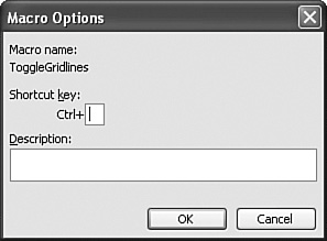
Listing 12.8. Procedures That Set and Reset a Key Combination Using the OnKey Method

 Sub SetKey()     Application.OnKey _         Key:="^{Del}", _         Procedure:="Chapter12.xls!DeleteAll" End Sub Sub DeleteAll()     Selection.Clear End Sub Sub ResetKey()     Application.OnKey _         Key:="^{Del}" End Sub 

Toggling Gridlines On and Off

If you find yourself regularly turning gridlines off and then back on for a particular window, it's a hassle to be constantly opening the Options dialog box to do this. For faster service, use the macro in Listing 12.9 and assign it to a toolbar button or keyboard shortcut.

Listing 12.9. A Macro That Toggles Gridlines On and Off

 Sub ToggleGridlines()     With ActiveWindow         .DisplayGridlines = Not .DisplayGridlines     End With End Sub 

Creating a Workbook with a Specified Number of Sheets

By default, Excel provides you with three worksheets in each new workbook. You can change the default number of sheets by selecting Tools, Options, displaying the General tab, and then adjusting the Sheets in New Workbook value. However, what if you want more control over the number of sheets in each new workbook? For example, a simple loan amortization model might require just a single worksheet, whereas a company budget workbook might require a dozen worksheets.

The macro in Listing 12.10 solves this problem by enabling you to specify the number of sheets you want in each new workbook.

Listing 12.10. A Macro That Creates a New Workbook with a Specified Number of Worksheets

 Sub NewWorkbookWithCustomSheets()     Dim currentSheets As Integer     With Application         currentSheets = .SheetsInNewWorkbook         .SheetsInNewWorkbook = InputBox("How many sheets do you want in the new workbook?", , 3)         Workbooks.Add         .SheetsInNewWorkbook = currentSheets     End With End Sub 

The value of the Sheets in New Workbook setting is given by the Application object's SheetsInNewWorkbook property. The macro first stores the current SheetsInNewWorkbook value in the currentSheets variable. Then the macro runs the InputBox function to get the number of required sheets (with a default value of 3), and this value is assigned to the SheetsInNewWorkbook property. Then the Workbooks.Add statement creates a new workbook (which will have the specified number of sheets) and the SheetsInNewWorkbook property is returned to its original value.

Automatically Sorting a Range After Data Entry

If you have a sorted range, you might find that the range requires resorting after data entry because the values on which the sort is based have changed. Rather than constantly invoking the Sort command, you can set up a macro that sorts the range automatically every time the relevant data changes.

As an example, consider the simple parts database shown in Figure 12.5. The range is sorted on the Gross Margin column (H), the values of which are determined using a formula that requires input from cells in columns E and G. In other words, each time a value in column E or G changes, the corresponding Gross Margin value changes. We want to keep the list sorted based on these changes.

Figure 12.5. The parts database range is sorted on the Gross Margin column (H).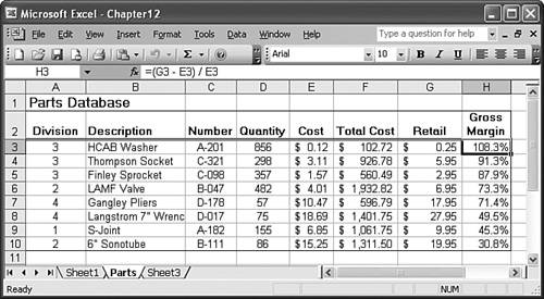

Listing 12.11 shows a couple of macros that serve to keep the range sorted automatically.

Listing 12.11. Two Macros That Keep the Parts Database Sorted Automatically

 Sub Auto_Open()     ThisWorkbook.Worksheets("Parts").OnEntry = "SortParts" End Sub Sub SortParts()     Dim currCell As Range     Set currCell = Application.Caller     If currCell.Column = 5 Or currCell.Column = 7 Then         Selection.Sort Key1:=Range("H1"), _                 Order1:=xlDescending, _                 Header:=xlYes, _                 OrderCustom:=1, _                 MatchCase:=False, _                 Orientation:=xlTopToBottom     End If End Sub 

Auto_Open is a macro that runs automatically when the workbook containing the code is opened. In this case, the statement sets the OnEntry event of the Parts worksheet to run the SortParts macro. The OnEntry event fires whenever data entry occurs in the specified object (in this case, the Parts worksheet).

The SortParts macro begins by examining the value of the Application object's Caller property, which returns a Range object that indicates which cell invoked the SortParts macro. In this context, Caller tells us in which cell the data entry occurred, and that cell address is stored in the currCell variable. Next, the macro checks currCell to see if the data entry occurred in either column E or column G. If so, the new value changes the calculated value in the Gross Margin column, so the range needs to be resorted. This is accomplished by running the Sort method, which sorts the range based on the values in column H.

Selecting A1 on All Worksheets

When you open an Excel file that you've worked on before, the cells or ranges that were selected in each worksheet when the file was last saved remain selected upon opening. This is handy behavior because it often enables you to resume work where you left off previously. However, when you've completed work on an Excel file, you may prefer to remove all the selections. For example, you might run through each worksheet and select cell A1 so that you or anyone else opening the file can start "fresh."

Selecting all the A1 cells manually is fine if the workbook has only a few sheets, but it can be a pain in a workbook that contains many sheets. Listing 12.12 presents a macro that selects cell A1 in all of a workbook's sheets.

Listing 12.12. A Macro That Selects Cell A1 on All the Sheets in the Active Workbook

 Sub SelectA1OnAllSheets()     Dim ws As Worksheet     '     ' Run through all the worksheets in the active workbook     '     For Each ws In ActiveWorkbook.Worksheets         '         ' Activate the worksheet         '         ws.Activate         '         ' Select cell A1         '         ws.[A1].Select     Next 'ws     '     ' Activate the first worksheet     '     ActiveWorkbook.Worksheets(1).Activate End Sub 

The macro runs through all the worksheets in the active workbook. In each case, the worksheet is first activated (you must activate a sheet before you can select anything on it), and then the Select method is called to select cell A1. The macro finishes by activating the first worksheet.

Selecting the "Home Cell" on All Worksheets

Many worksheets have a "natural" starting point, which could be a model's first data entry cell or a cell that displays a key result. In such a case, rather than selecting cell A1 on all the worksheets, you might prefer to select each of these "home cells."

One way to do this is to add a uniform comment to each home cell. For example, you could add the comment Home Cell. Having done that, you can then use the macro in Listing 12.13 to select all these home cells.

Listing 12.13. A Macro That Selects the "Home Cell" on All the Sheets in the Active Workbook

 Sub SelectHomeCells()     Dim ws As Worksheet     Dim c As Comment     Dim r As Range     '     ' Run through all the worksheets in the active workbook     '     For Each ws In ActiveWorkbook.Worksheets         '         ' Activate the worksheet         '         ws.Activate         '         ' Run through the comments         '         For Each c In ws.Comments             '             ' Look for the "Home Cell" comment             '             If InStr(c.Text, "Home Cell") <> 0 Then                 '                 ' Store the cell as a Range                 '                 Set r = c.Parent                 '                 ' Select the cell                 '                 r.Select             End If         Next 'c     Next 'ws     '     ' Activate the first worksheet     '     ActiveWorkbook.Worksheets(1).Activate End Sub 

The SelectHomeCells procedure is similar to the SelectA1OnAllSheets procedure from Listing 12.12. That is, the main loop runs through all the sheets in the active workbook and activates each worksheet in turn. In this case, however, another loop runs through each worksheet's Comments collection. The Text property of each Comment object is checked to see if it includes the phrase Home Cell. If so, the cell containing the comment is stored in the r variable (using the Comment object's Parent property) and then the cell is selected.

Selecting the Named Range That Contains the Active Cell

It's often handy to be able to select the name range that contains the current cell (for example, to change the range formatting). If you know the name of the range, you need only select it from the Name box. However, in a large model or a workbook that you're not familiar with, it may not be obvious which name to choose. Listing 12.14 shows a function and procedure that will handle this chore for you.

Listing 12.14. A Function and Procedure That Determine and Select the Named Range Containing the Active Cell

 Function GetRangeName(r As Range) As String     Dim n As Name     Dim rtr As Range     Dim ir As Range     '     ' Run through all the range names in the active workbook     '     For Each n In ActiveWorkbook.Names         '         ' Get the name's range         '         Set rtr = n.RefersToRange         '         ' See if the named range and the active cell's range intersect         '         Set ir = Application.Intersect(r, rtr)         If Not ir Is Nothing Then             '             ' If they intersect, then the active cell is part of a             ' named range, so get the name and exit the function             GetRangeName = n.Name             Exit Function         End If     Next 'n     '     ' If we get this far, the active cell is not part of a named range,     ' so return the null string     '     GetRangeName = "" End Function Sub SelectCurrentNamedRange()     Dim r As Range     Dim strName As String     '     ' Store the active cell     '     Set r = ActiveCell     '     ' Get the name of the range that contains the cell, if any     '     strName = GetRangeName(r)     If strName <> "" Then         '         ' If the cell is part of a named range, select the range         '         Range(strName).Select     End If End Sub 

The heart of Listing 12.14 is the GetrangeName function, which takes a range as an argument. The purpose of this function is to see whether the passed rangeris part of a named range and if so, to return the name of that range. The function's main loop runs through each item in the active workbook's Names collection. For each name, the RefersToRange property returns the associated range, which the function stores in the rtr variable. The function then uses the Intersect method to see if the ranges r and rtr intersect. If they do, it means that r is part of the named range (because, in this case, r is just a single cell), so GetrangeName returns the range name. If no intersection is found for any name, the function returns the null string (""), instead.

The SelectCurrentNamedRange procedure makes use of the GetrangeName function. The procedure stores the active cell in the r variable and then passes that variable to the GeTRangeName function. If the return value is not the null string, the procedure selects the returned range name.

Saving All Open Workbooks

In Word, if you hold down Shift and then drop down the File menu, the Save command changes to Save All; selecting this command saves all the open documents. Unfortunately, this very useful feature isn't available in Excel. Listing 12.15 presents a macro named SaveAll that duplicates Word's Save All command.

Listing 12.15. A Macro That Saves All Open Workbooks

 Sub SaveAll()     Dim wb As Workbook     Dim newFilename As Variant     '     ' Run through all the open workbooks     '     For Each wb In Workbooks         '         ' Has the workbook been saved before?         '         If wb.Path <> "" Then             '             ' If so, save it             '             wb.Save         Else             '             ' If not, display the Save As dialog box             ' to get a path and filename for the workbook             '             newFilename = Application.GetSaveAsFilename(FileFilter:= _                           "Microsoft Office Excel Workbook (*.xls), *.xls")             '             ' Did the user click Cancel?             '             If newFilename <> False Then                 '                 ' If not, save the workbook using the                 ' specified path and filename                 '                 wb.SaveAs fileName:=newFilename             End If         End If     Next 'wb End Sub 

The main loop in the SaveAll macro runs through all the open workbooks. For each workbook, the loop first checks the Path property to see if it returns the null string (""). If not, it means the workbook has been saved previously, so the macro runs the Save method to save the file. If Path does return the null string, it means we're saving the workbook for the first time. In this case, the macro runs the GetSaveAsFilename method. It displays the Save As dialog box so that the user can select a save location and filename, which are stored in the newFilename variable. If this variable's value is False, it means the user clicked Cancel in the Save As dialog box, so the macro skips the file; otherwise, the macro saves the workbook using the specified path and filename.