Analyzing Data with Lists

Excel's forte is spreadsheet work, but its row-and-column layout also makes it a natural flat-file database manager. In Excel, a list is a collection of related information with an organizational structure that makes it easy to find or extract data from its contents. Specifically, a list is a worksheet range that has the following properties:

FieldA single type of information, such as a name, an address, or a phone number. In Excel lists, each column is a field.
Field valueA single item in a field. In an Excel list, the field values are the individual cells.
Field nameA unique name you assign to every list field (worksheet column). These names are always found in the first row of the list.
RecordA collection of associated field values. In Excel lists, each row is a record.
List rangeThe worksheet range that includes all the records, fields, and field names of a list.

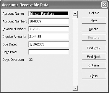
For example, suppose that you want to set up an accounts-receivable list. A simple system would include information such as account name, account number, invoice number, invoice amount, due date, and date paid, as well as a calculation of the number of days overdue. Figure 2.22 shows how this system would be implemented as an Excel list.

Figure 2.22. Accounts-receivable data in an Excel worksheet.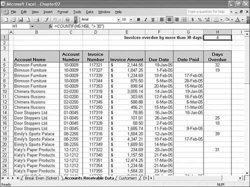

Excel lists don't require elaborate planning, but you should follow a few guidelines for best results. Here are some pointers:

Always use the top row of the list for the column labels.
Field names must be unique, and they must be text or text formulas. If you need to use numbers, format them as text.
Some Excel commands can automatically identify the size and shape of a list. To avoid confusing such commands, try to use only one list per worksheet. If you have multiple related lists, include them in other worksheets in the same workbook.
If you have nonlist data in the same worksheet, leave at least one blank row or column between the data and the list. This helps Excel to identify the list automatically.
Excel has a command that enables you to filter your list data to show only records that match certain criteria. (See "Filtering List Data," later in this chapter, for details.) This command works by hiding rows of data. Therefore, if the same worksheet contains nonlist data that you need to see or work with, don't place this data to the left or right of the list.

Converting a Range to a List

Excel has a number of commands that enable you to work efficiently with list data. To take advantage of these commands, you must convert your data from a normal range to a list by following these steps:

1.	Click any cell within the range that you want to convert to a list.
2.	Choose Data, List, Create List (or press Ctrl+L). Excel displays the Create List dialog box.
3.	The Where Is the Data for Your List? box should already show the correct range coordinates. If not, enter the range coordinates or select the range directly on the worksheet.
4.	If your range has column headers in the top row (as it should), make sure the My List Has Headers check box is activated.
5.	Click OK.

When you convert a range to a list, Excel makes three changes to the range, as shown in Figure 2.23:

It displays a border around the list.
It adds drop-down arrows to each field header.
It displays the List toolbar whenever you select a cell within the list.

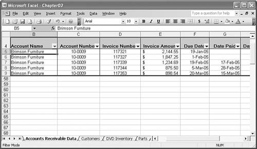
Figure 2.23. The accounts-receivable data converted to a list.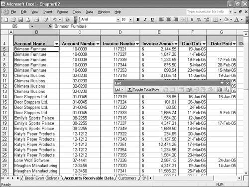

If you ever need to change the list back to a range, select a cell within the list and choose Data, List, Convert to Range.

Basic List Operations

After you've converted the range to a list, you can start working with the data. Following is a quick look at some basic list operations:

Adding a new record anywhere in the listSelect any cell in a record below which you want to add the new record. In the List toolbar, choose List, Insert, Row. Excel inserts a blank row above the selected cell into which you can enter the new data.

Adding a new record at the bottom of the listAfter you have inserted a row, you'll see an asterisk (*) in the first field below the last record in the list. This is the new record symbol, and it means that you can use this row to add a new record to the list.

Turning Off Excel's Warning Dialog

As soon as you start entering data into the new record, Excel displays a dialog box to tell you that it has inserted a row. You can avoid being pestered by this bit of obvious news by clicking the Do Not Display This Dialog Again check box.

Deleting a recordSelect any cell in the record you want to delete. In the List toolbar, choose List, Delete, Row.

Working with a record using a data formChoose Data, Form (or, on the List toolbar, choose List, Form). This displays the list's data form, which is a dialog box that enables you to add, edit, delete, and find list records quickly (see Figure 2.24). To add a record to the list, click New and enter the data into the blank fields. To edit a record, use the scrollbar to select it and then edit the fields. To delete a record, use the scrollbar to select it, click Delete, and then click OK to confirm the deletion.

Figure 2.24. The data form for the accounts-receivable list.

Invalid List Error

When you select the Form command, you may see a dialog box warning you that the Database or list range is not valid. This usually means that your workbook has an existing range named Database. Select Insert, Name, Define, select the Database name, and then click Delete.

Finding a record using criteriaDisplay the data form, click Criteria, and then enter the criteria you want to use in the corresponding field. For example, if you want to find a record where the Invoice Amount field is greater than $1,000, enter >1000 in the data form's Invoice Amount box. Use the Find Prev and Find Next buttons to scroll through the records that match the criteria.

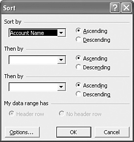
Sorting a List

One of the advantages of a list is that you can rearrange the records so that they're sorted alphabetically or numerically. This feature enables you to view the data in order by customer name, account number, part number, or any other field. You even can sort on multiple fields, which would enable you, for example, to sort a client list by state and then by name within each state.

The following procedure shows you how to sort a list:

Select a cell inside the list.

Choose List, Sort on the List toolbar. Excel displays the Sort dialog box, shown in Figure 2.25.

Figure 2.25. Use the Sort dialog box to sort the list on one or more fields.

Use the Sort By list to select the field you want to use for the overall order for the sort.

(Optional) If you want to sort the data on more than one field, use one or both of the Then By lists to select the field or fields you want to use.

Sorting and Formulas

Be careful when you sort list records that contain formulas. If the formulas use relative addresses that refer to cells outside their own record, the new sort order might change the references and produce erroneous results. If your list formulas must refer to cells outside the list, be sure to use absolute addresses.

For each sort field, select either Ascending or Descending.

Excel's Sorting Order

How Excel sorts the list depends on the data. Here's the order Excel uses in an ascending sort:

Type (in Order of Priority)	Order
Numbers	Largest negative to largest positive
Text	Space!" # $ % & ' ( ) * + , - . / 0 through 9 (when formatted as text) :;< = > ? @ A through Z (Excel ignores case) [ \ ] ^_ ' {,} ~
Logical	`FALSE` before `trUE`
Error	All error values are equal
Blank	Always sorted last (ascending or descending)

(Optional) Choose Options to specify one or more of the following sort controls:

First Key Sort OrderSets a custom sort order (using an AutoFill list) for the field you chose in the Sort By list. For example, to sort by the days of the week, select the Sun, Mon, Tue option.

Case SensitiveActivate this option to have Excel differentiate between uppercase and lowercase during sorting. In an ascending sort, for example, lowercase letters are sorted before uppercase letters.

OrientationExcel normally sorts list rows (the Sort Top to Bottom option). To sort list columns, activate Sort Left to Right.

Click OK. Excel sorts the range.

Custom AutoFill Lists

You're not stuck with only the few AutoFill lists that Excel recognizes out of the box. You're free to define your own AutoFill lists. To start, choose Tools, Options, click the Custom Lists tab, and then click New List. Type an item from your list into the List Entries box, press Enter, and then repeat for each item. (Make sure that you add the items in the order in which you want them to appear in the series.) Click Add to add the list to the Custom Lists box, and then click OK to return to the worksheet.

Sorting on More Than Three Keys

You're not restricted to sorting on only three fields in an Excel list. By performing consecutive sorts, you can sort on any number of fields. For example, suppose that you want to sort a customer list by the following fields (in order of importance): Region, State, City, ZIP Code, and Name. To use five fields, you must perform two consecutive sorts. The first sort uses the three least important fields: City, ZIP Code, and Name. Of these three, City is the most important, so it's selected in the Sort By field; ZIP Code is selected in the first Then By field, and Name is selected in the second Then By field. When this sort is complete, you must run a second sort using the remaining keys, Region and State. Select Region in the Sort By list and State in the first Then By list.

By running multiple sorts and always using the least important fields first, you can sort on as many fields as you like.

Sorting a List in Natural Order

It's often convenient to see the order in which records were entered into a list, or the natural order of the data. Normally, you can restore a list to its natural order by choosing Edit, Undo Sort immediately after a sort.

Unfortunately, after several sort operations, it's no longer possible to restore the natural order. The solution is to create a new field, called, for example, Record, in which you assign consecutive numbers as you enter the data. The first record is 1, the second is 2, and so on. To restore the list to its natural order, you sort on the Record field.

Add the Record Field Up Front

The Record field will work only if you add it either before you start inserting new records in the list or before you've irrevocably sorted the list. Therefore, when planning any list, you might consider always including a Record field just in case you need it.

Follow these steps to add a new field to the list:

1.	Select a cell in the field to the right of where you want the new field inserted.
2.	In the List toolbar, choose List, Insert, Column. Excel inserts the column.
3.	Rename the column header to the field name you want to use.

Figure 2.26 shows the Accounts Receivable list with a Record field added and the record numbers inserted.

Figure 2.26. The Record field tracks the order in which records are added to a list.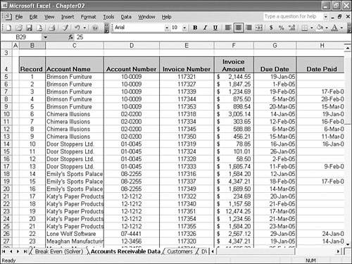

Calculating the Next Record Number

If you're not sure how many records are in the list, and if the list isn't sorted in natural order, you might not know which record number to use next. To avoid guessing or searching through the entire Record field, you can generate the record numbers automatically using the MAX() function. Click the formula bar and type (but don't confirm) the following:

 =MAX(Column:Column)

Replace Column with the letter of the column that contains the record number (for example, MAX(B:B) for the list in Figure 2.26). Now highlight the formula and press F9. Excel displays the formula result that will be the highest record number used so far. Therefore, your next record number will be one more than the calculated value.

Sorting on Part of a Field

Excel performs its sorting chores based on the entire content of each cell in the field. This method is fine for most sorting tasks, but occasionally you'll need to sort on only part of a field. For example, your list might have a ContactName field that contains a first name and then a last name. Sorting on this field orders the list by each person's first name, which is probably not what you want. To sort on the last name, you need to create a new column that extracts the last name from the field. You can then use this new column for the sort.

Excel's text functions make it easy to extract substrings from a cell. In this case, assume that each cell in the ContactName field has a first name, followed by a space, followed by a last name. Your task is to extract everything after the space, and the following formula does the job (assuming that the name is in cell D2):

 =RIGHT(D2, LEN(D2) - FIND(" ", D2))

Figure 2.27 shows this formula in action. Column D contains the names, and column A contains the formula to extract the last name. I sorted on column A to order the list by last name.

Figure 2.27. To sort on part of a field, use Excel's text functions to extract the string you need for the sort.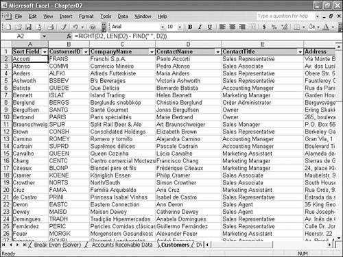

Hiding the Extra Sort Field

If you'd rather not have the extra sort field (column A in Figure 2.27) cluttering the list, you can hide it by selecting a cell in the field and choosing Format, Column, Hide. Fortunately, you don't have to unhide the field to sort on it because Excel still includes the field in the Sort By list.

Sorting Without Articles

Lists that contain field values starting with articles (A, An, and The) can throw off your sorting. To fix this problem, you can borrow the technique from the preceding section and sort on a new field in which the leading articles have been removed. As before, you want to extract everything after the first space, but you can't just use the same formula because not all the titles have a leading article. You need to test for a leading article using the following OR() function:

 OR(LEFT(A2,2) = "A ", LEFT(A2,3) = "An ", LEFT(A2,4) = "The ")

Here I'm assuming that the text being tested is in cell A2. If the left two characters are A, or the left three characters are An, or the left four characters are The, this function returns TRUE (that is, you're dealing with a title that has a leading article).

Now you need to package this OR() function inside an IF() test. If the OR() function returns trUE, the command should extract everything after the first space; otherwise, it should return the entire title. Here it is (Figure 2.28 shows the formula in action):

 =IF( OR(LEFT(A2,2) = "A ", LEFT(A2,3) = "An ", LEFT(A2,4) = "The "), RIGHT(A2, LEN(A2) - FIND(" ", A2, 1)), A2)

Figure 2.28. A formula that removes leading articles for proper sorting.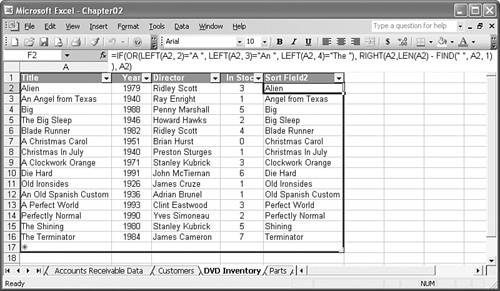

Filtering List Data

One of the biggest problems with large lists is that it's often hard to find and extract the data you need. Sorting can help, but in the end, you're still working with the entire list. What you need is a way to define the data that you want to work with and then have Excel display only those records onscreen. This action is called filtering your data. Fortunately, Excel offers several techniques that get the job done.

Using AutoFilter to Filter a List

Excel's AutoFilter feature makes filtering out subsets of your data as easy as selecting an option from a drop-down list. In fact, that's literally what happens. When you convert a range to a list, Excel automatically turns on AutoFilter, which is why you see drop-down arrows in the cells containing the list's column labels. (You can toggle AutoFilter off and on by choosing Data, Filter, AutoFilter.) Clicking one of these arrows displays a list of all the unique entries in the column. Figure 2.29 shows the drop-down list for the Account Name field in an Accounts Receivable database.

Figure 2.29. For each list field, AutoFilter adds drop-down lists that contain only the unique entries in the column.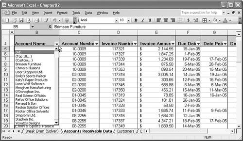

If you click an item in one of these AutoFilter lists, Excel takes the following actions:

It displays only those records that include the item in that field. For example, Figure 2.30 shows the resulting records when the item Brimson Furniture is selected from the list attached to the Account Name column. The other records are hidden and can be retrieved whenever you need them.

Figure 2.30. Clicking an item in an AutoFilter drop-down list displays only records that include the item in the field.

Watch for Data Outside the Table

Because Excel hides the rows that don't meet the criteria, you shouldn't place any important data either to the left or to the right of the list.
It changes the color of the column's drop-down arrow. This indicates which column you used to filter the list.
It displays Filter Mode in the status bar.

To continue filtering the data, you can select an item from one of the other lists. For example, you could choose a date from the Due Date list to see only those Brimson Furniture invoices due on that date.

AutoFilter Criteria Options

The items you see in each drop-down list are called the filter criteria. Besides selecting specific criteria (such as an account name), you have the following choices in each drop-down list:

AllRemoves the filter criterion for the column. If you've selected multiple criteria, you can remove all the filter criteria and display the entire list by choosing Data, Filter, Show All.
Top 10In a numeric or date field, displays the Top 10 AutoFilter dialog box, as shown in Figure 2.31. The left drop-down list has two choices, Top or Bottom. The center spin box enables you to choose a number. The right drop-down list has two choices, Items and Percent. For example, if you choose the default choices (Top, 10, and Items), AutoFilter displays the records that have the 10 highest values in the current field.

Figure 2.31. Use the Top 10 AutoFilter dialog box to filter your records based on values in the current field.
CustomEnables you to enter more sophisticated criteria. For details, see the next section.

Setting Up Custom AutoFilter Criteria

In its basic form, AutoFilter enables you to select only a single item from each column drop-down list. AutoFilter's custom filter criteria, however, give you a way to select multiple items. In the Accounts Receivable list, for example, you could use custom criteria to display all the invoices with the following:

An account number that begins with 07
A due date in January
An amount between $1,000 and $5,000
An account name of either Refco Office Solutions or Brimson Furniture

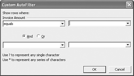
Before you learn the steps required to create a custom AutoFilter criterion, let's go through an overview of what happens. When you click the Custom option in an AutoFilter drop-down list, Excel displays the Custom AutoFilter dialog box, shown in Figure 2.32.

Figure 2.32. Use the Custom AutoFilter dialog box to enter your custom criteria.

You use the two drop-down lists across the top to set up the first part of your criterion. The list on the left contains a list of Excel's comparison operators (such as Equals and Is Greater Than). The combo box on the right enables you to select a unique item from the field or enter your own value. For example, if you want to display invoices with an amount greater than or equal to $1,000, click the Is Greater Than or Equal operator and enter 1000 into the text box.

For text fields, you can also use wildcard characters to substitute for one or more characters. Use the question mark (?) wildcard to substitute for a single character. For example, if you enter sm?th, Excel finds both Smith and Smyth. To substitute for groups of characters, use the asterisk (*). For example, if you enter *carolina, Excel finds all the entries that end with "carolina."

Including Wildcards

To include a wildcard as part of the criteria, precede the character with a tilde (~). For example, to find OVERDUE?, enter OVERDUE~?.

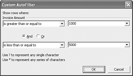
You can create compound criteria by clicking the And or Or buttons and then entering another criterion in the bottom two drop-down lists. Use And when you want to display records that meet both criteria; use Or when you want to display records that meet at least one of the two criteria.

For example, to display invoices with an amount greater than or equal to $1,000 and less than or equal to $5,000, you fill in the dialog box as shown in Figure 2.33.

Figure 2.33. A compound criterion that displays the records with invoice amounts between $1,000 and $5,000.

The following procedure takes you through the official steps to set up a custom AutoFilter criterion:

1.	Click Custom in the drop-down list attached to the column you want to work with. Excel displays the Custom AutoFilter dialog box.
2.	Click a comparison operator and enter a value for the first part of the criterion. If you don't want to create a compound criterion, skip to step 5.
3.	Click either the And option or the Or option, as appropriate.
4.	Click a comparison operator and enter a value for the second part of the criterion.
5.	Click OK. Excel filters the list.

Showing Filtered Records

When you need to redisplay records that have been filtered via AutoFilter, use any of the following techniques:

To display the entire list and remove AutoFilter's drop-down arrows, deactivate the Data, Filter, AutoFilter command.
To display the entire list without removing the AutoFilter drop-down arrows, choose Data, Filter, Show All.
To remove the filter on a single field, display that field's AutoFilter drop-down list and click the All option.

Using Complex Criteria to Filter a List

The AutoFilter should take care of most of your filtering needs, but it's not designed for heavy-duty work. For example, AutoFilter can't handle the following Accounts Receivable criteria:

Invoice amounts greater than $100, less than $1,000, or greater than $10,000
Account numbers that begin with 01, 05, or 12
Days overdue greater than the value in cell J1

To work with these more sophisticated requests, you need to use complex criteria.

Setting Up a Criteria Range

Before you can work with complex criteria, you must set up a criteria range. A criteria range has some or all of the list field names in the top row, with at least one blank row directly underneath. You enter your criteria in the blank row below the appropriate field name, and Excel searches the list for records with field values that satisfy the criteria. This setup gives you two major advantages over AutoFilter:

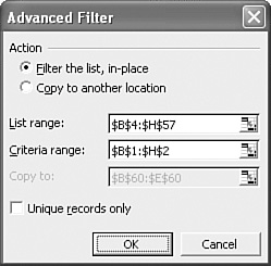
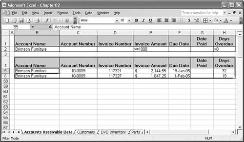
By using either multiple rows or multiple columns for a single field, you can create compound criteria with as many terms as you like.
Because you're entering your criteria in cells, you can use formulas to create computed criteria.

You can place the criteria range anywhere on the worksheet outside the list range. The most common position, however, is a couple of rows above the list range. Figure 2.34 shows the Accounts Receivable list with a criteria range. As you can see, the criteria are entered in the cell below the field name. In this case, the displayed criteria will find all Brimson Furniture invoices that are greater than or equal to $1,000 and that are overdue (that is, invoices that have a value greater than 0 in the Days Overdue field).

Figure 2.34. Set up a separate criteria range (B1:D2, in this case) to enter complex criteria.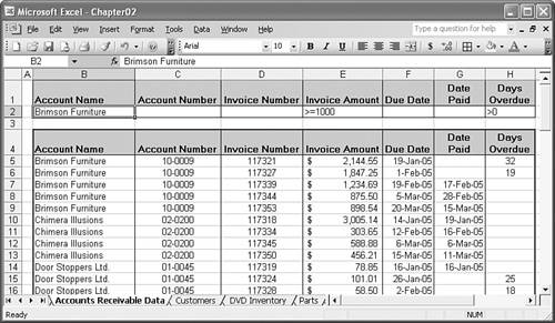

Filtering a List with a Criteria Range

After you've set up your criteria range, you can use it to filter the list. The following procedure takes you through the basic steps:

Copy the list field names that you want to use for the criteria and paste them into the first row of the criteria range. If you'll be using different fields for different criteria, consider copying all your field names into the first row of the criteria range.

Use Formulas for Criteria Field Name

The only problem with copying the field names to the criteria range is that if you change a field name, you must change it in two places (that is, in the list and in the criteria). So, instead of just copying the names, you can make the field names in the criteria range dynamic by using a formula to set each criteria field name equal to its corresponding list field name. For example, you could enter =B4 into cell B1 of Figure 2.34.

Below each field name in the criteria range, enter the criteria you want to use.

Select a cell in the list, and then choose Data, Filter, Advanced Filter. Excel displays the Advanced Filter dialog box, shown in Figure 2.35.

Figure 2.35. Use the Advanced Filter dialog box to select your list and criteria ranges.

The List Range text box should contain the list range (if you selected a cell in the list beforehand). If it doesn't, activate the text box and select the list (including the field names).

In the Criteria Range text box, select the criteria range (again, including the field names you copied).

To avoid including duplicate records in the filter, activate the Unique Records Only check box.

Click OK. Excel filters the list to show only those records that match your criteria (see Figure 2.36).

Figure 2.36. Set up a separate criteria range (B1:H2, in this case) to enter complex criteria.

Entering Compound Criteria

To enter compound criteria in a criteria range, use the following guidelines:

To find records that match all the criteria, enter the criteria on a single row.
To find records that match one or more of the criteria, enter the criteria in separate rows.

Finding records that match all the criteria is equivalent to activating the And button in the Custom AutoFilter dialog box. The sample criteria shown earlier in Figure 2.34 match records with the account name Brimson Furniture and an invoice amount greater than $1,000 and a positive number in the Days Overdue field. To narrow the displayed records, you can enter criteria for as many fields as you like.

Using a Field Multiple Times in a Criteria Range

You can use the same field name more than once in compound criteria. To do this, include the appropriate field multiple times in the criteria range and enter the appropriate criteria below each label.

Finding records that match at least one of several criteria is equivalent to activating the Or button in the Custom AutoFilter dialog box. In this case, you need to enter each criterion on a separate row. For example, to display all invoices with amounts greater than or equal to $10,000 or that are more than 30 days overdue, you would set up your criteria as shown in Figure 2.37.

Figure 2.37. To display records that match one or more of the criteria, enter the criteria in separate rows.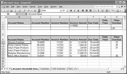

Don't Include Blank Rows

Don't include any blank rows in your criteria range because blank rows throw off Excel when it tries to match the criteria.

Entering Computed Criteria

The fields in your criteria range aren't restricted to the list fields. You can create computed criteria that use a calculation to match records in the list. The calculation can refer to one or more list fields, or even to cells outside the list, and must return either trUE or FALSE. Excel selects records that return trUE.

To use computed criteria, add a column to the criteria range and enter the formula in the new field. Make sure that the name you give the criteria field is different from any field name in the list. When referencing the list cells in the formula, use the first row of the list. For example, to select all records in which the Date Paid is equal to the Due Date in the accounts receivable list, enter the following formula:

 =G5=F5

Note the use of relative addressing. If you want to reference cells outside the list, use absolute addressing.

Creating Compound Computed Criteria

Use Excel's AND, OR, and NOT functions to create compound computed criteria. For example, to select all records in which the Days Overdue value is less than 90 and greater than 31, type the following:

 =AND(H5<90, H5>31)

Figure 2.38 shows a more complex example. The goal is to select all records whose invoices were paid after the due date. The new criterionnamed Late Payerscontains the following formula:

 =IF(ISBLANK(G5), FALSE(), G5 > F5)

Figure 2.38. Use a separate criteria range column for calculated criteria.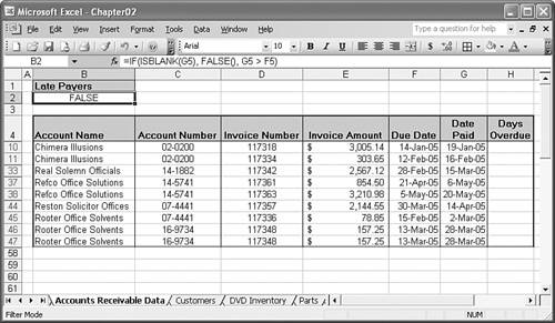

If the Date Paid field (column G) is blank, the invoice hasn't been paid, so the formula returns FALSE. Otherwise, the logical expression G5 > F5 is evaluated. If the Date Paid (column G) is greater than the Due Date field (column F), the expression returns trUE and Excel selects the record. In Figure 2.38, the Late Payers cell (B2) displays FALSE because the formula evaluates to FALSE for the first row in the list.

Summarizing List Data

Because a list is just a special kind of worksheet range, you can analyze list data using many of the same methods you use for regular worksheet cells. Typically, this task involves using formulas and functions to answer questions and produce results. To make your analysis chores easier, Excel enables you to create automatic subtotals that can give you instant subtotals, averages, and more. Excel goes one step further by also offering many list-specific functions. These functions work with entire lists or subsets defined by a criteria range. The rest of this chapter shows you how to use all these tools to analyze and summarize your data.

Creating Automatic Subtotals

Automatic subtotals enable you to summarize your sorted list data quickly. For example, if you have a list of invoices sorted by account name, you can use automatic subtotals to give you the following information for each account:

The total number of invoices
The sum of the invoice amounts
The average invoice amount
The maximum number of days an invoice is overdue

You can do all this and more without entering a single formula. Excel does the calculations and enters the results automatically. You also can just as easily create grand totals that apply to the entire list.

More Than Just Subtotals

The term automatic subtotal is somewhat of a misnomer because you can summarize more than totals. For this topic, at least, think of a subtotal as any summary calculation.

Setting Up a List for Automatic Subtotals

Excel calculates automatic subtotals based on data groupings in a selected field. For example, if you ask for subtotals based on account name, Excel runs down the account name column and creates a new subtotal each time the name changes. To get useful summaries, then, you need to sort the list on the field containing the data groupings you're interested in. Figure 2.39 shows the Accounts Receivable database sorted by account name. If you subtotal the Account Name field, you get summaries for Brimson Furniture, Chimera Illusions, Door Stoppers Ltd., and so on.

Figure 2.39. A sorted list ready for displaying subtotals.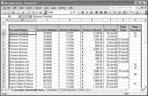

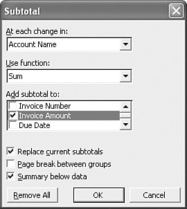
Subtotals for Filtered Lists

If you want to display subtotals for a filtered list, be sure to filter the list before sorting it (as described earlier in this chapter).

Displaying Subtotals

To subtotal a list, follow these steps:

1.	If you haven't already done so, sort your list according to the groupings you want to use for the subtotals.
2.	Convert the list to a normal range by choosing Data, List, Convert to Range, and then choosing Yes when Excel asks you to confirm.
3.	Choose Data, Subtotals to display the Subtotal dialog box, shown in Figure 2.40. Figure 2.40. You use the Subtotal dialog box to create subtotals for your list.
4.	Enter the options you want to use for the subtotals: At Each Change InThis box contains the field names for your list. Click the field you want to use to group the subtotals. Use FunctionSelect the function you want to use in the calculations. Excel gives you 11 choices, including Sum, Count, Average, Max, and Min. Add Subtotal ToThis is a list of check boxes for each field. Activate the appropriate check boxes for the fields you want to subtotal. Replace Current SubtotalsActivate this check box to display new subtotal rows. To add to the existing rows, deactivate this option. Page Break Between GroupsIf you intend to print the summary, activate this check box to insert a page break between each grouping. Summary Below DataDeactivate this check box if you want the subtotal rows to appear above the groupings.
5.	Click OK. Excel calculates the subtotals and enters them into the list.

Figure 2.41 shows the Accounts Receivable list with the Invoice Amount field subtotaled.

Figure 2.41. A list showing Invoice Amount subtotals for each Account Name.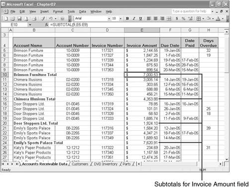

Adding More Subtotals

You can add any number of subtotals to the current summary. The following procedure shows you what to do:

1.	Choose Data, Subtotals to display the Subtotal dialog box.
2.	Enter the options you want to use for the new subtotal.
3.	Deactivate the Replace Current Subtotals check box.
4.	Click OK. Excel calculates the new subtotals and adds them to the list.

For example, Figure 2.42 shows the Accounts Receivable list with two new subtotals that count the invoices and display the maximum number of days overdue.

Figure 2.42. You can use multiple subtotals in a list.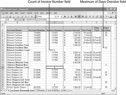

Removing Subtotals

To remove the subtotals from a list, choose Data, Subtotals to display the Subtotal dialog box, and then click Remove All.

Excel's List Functions

To get more control over your list analysis, you can use Excel's list functions. These functions are the same as those used in subtotals, but they have the following advantages:

You can enter the functions into any cell in the worksheet.
You can specify the range the function uses to perform its calculations.
You can enter criteria or reference a criteria range to perform calculations on subsets of the list.

About List Functions

To illustrate the list functions, consider an example. If you want to calculate the sum of a list field, for instance, you can enter SUM(range), and Excel produces the result. If you want to sum only a subset of the field, you must specify as arguments the particular cells to use. For lists containing hundreds of records, however, this process is impractical. (It's also illegal, for two reasons: Excel allows a maximum of 30 arguments in the SUM() function, and it allows a maximum of 255 characters in a cell entry.)

The solution is to use DSUM(), which is the list equivalent of the SUM() function. The DSUM() function takes three arguments: a list range, a field name, and a criteria range. DSUM() looks at the specified field in the list and sums only records that match the criteria in the criteria range.

The list functions come in two varieties: those that don't require a criteria range and those that do.

List Functions That Don't Require a Criteria Range

Excel has two list functions that enable you to specify the criteria as an argument rather than a range: COUNTIF() and SUMIF().

Using `COUNTIF()`

The COUNTIF() function counts the number of cells in a range that meet a single criterion:

 COUNTIF(range, criteria)

`range`	The range of cells to use for the count.
`criteria`	The criteria, entered as text, that determines which cells to count. Excel applies the criterion to `range`.

For example, Figure 2.43 shows a COUNTIF() function that calculates the total number of invoices that are more than 30 days overdue.

Figure 2.43. Use `COUNTIF()` to count the cells that meet a criterion.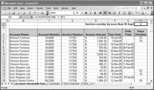

Using `SUMIF()`

The SUMIF() function is similar to COUNTIF(), except that it sums the range cells that meet its criterion:

 SUMIF(range, criteria [, sum_range])

`range`	The range of cells to use for the criterion.
`criteria`	The criteria, entered as text, that determines which cells to sum. Excel applies the criteria to `range`.
`sum_range`	The range from which the sum values are taken. Excel sums only those cells in `sum_range` that correspond to the cells in `range` and meet the criterion. If you omit `sum_range`, Excel uses `range` for the sum.

Figure 2.44 shows a Parts database. The SUMIF() function in cell F16 sums the total cost (F7:F14) for the parts where Division (A7:A14) is equal to 3.

Figure 2.44. Use `SUMIF()` to sum cells that meet a criterion.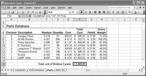

List Functions That Require a Criteria Range

The remaining list functions require a criteria range. These functions take a little longer to set up, but the advantage is that you can enter compound and computed criteria.

All these functions have the following format:

 Dfunction(database, field, criteria)

`Dfunction`	The function name, such as `DSUM` or `DAVERAGE`.
`database`	The range of cells that make up the list you want to work with. You can use either a range name, if one is defined, or the range address.
`field`	The name of the field on which you want to perform the operation. You can use either the field name or the field number as the argument (in which the leftmost field is field number 1, the next field is field number 2, and so on). If you use the field name, enclose it in quotation marks (for example, `"Total Cost"`).
`criteria`	The range of cells that hold the criteria you want to work with. You can use either a range name, if one is defined, or the range address.

Operating on Every Record

To perform an operation on every record in the list, leave all the criteria fields blank. This causes Excel to select every record in the list.

Table 2.1 summarizes the list functions.

Table 2.1. Excel's List Functions
Function	Description
`DAVERAGE()`	Returns the average of the matching records in a specified field.
`DCOUNT()`	Returns the count of the matching records.
`DCOUNTA()`	Returns the count of the nonblank matching records.
`DGET()`	Returns the value of a specified field for a single matching record.
`DMAX()`	Returns the maximum value of a specified field for the matching records.
`DMIN()`	Returns the minimum value of a specified field for the matching records.
`DPRODUCT()`	Returns the product of the values of a specified field for the matching records.
`DSTDEV()`	Returns the estimated standard deviation of the values in a specified field if the matching records are a sample of the population.
`DSTDEVP()`	Returns the standard deviation of the values of a specified field if the matching records are the entire population.
`DSUM()`	Returns the sum of the values of a specified field for the matching records.
`DVAR()`	Returns the estimated variance of the values of a specified field if the matching records are a sample of the population.
`DVARP()`	Returns the variance of the values of a specified field if the matching records are the entire population.

You enter list functions the same way you enter any other Excel function. You type an equal sign (=) and then enter the functioneither by itself or combined with other Excel operators in a formula. The following examples all show valid list functions:

 =DSUM(A6:H14, "Total Cost", A1:H3) =DSUM(List, "Total Cost", Criteria) =DSUM(AR_List, 3, Criteria) =DSUM(1993_Sales, "Sales", A1:H13)

The next two sections provide examples of the DAVERAGE() and DGET() list functions.

Using `DAVERAGE()`

The DAVERAGE() function calculates the average field value in the database records that match the criteria. In the Parts database, for example, suppose that you want to calculate the average gross margin for all parts assigned to Division 2. You set up a criteria range for the Division field and enter 2, as shown in Figure 2.45. You then enter the following DAVERAGE() function (see cell H3):

 =DAVERAGE(A6:H14, "Gross Margin", A2:A3)

Figure 2.45. Use `DAVERAGE()` to calculate the field average in the matching records.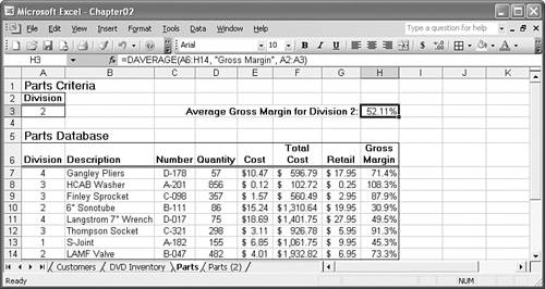

Using `DGET()`

The DGET() function extracts the value of a single field in the database records that match the criteria. If there are no matching records, DGET() returns #VALUE!. If there is more than one matching record, DGET() returns #NUM!.

DGET() typically is used to query the list for a specific piece of information. For example, in the Parts list, you might want to know the cost of the Finley Sprocket. To extract this information, you would first set up a criteria range with the Description field and enter Finley Sprocket. You would then extract the information with the following formula (assuming that the list and criteria ranges are named Database and Criteria, respectively):

 =DGET(Database, "Cost", Criteria)

A more interesting application of this function would be to extract the name of a part that satisfies a certain condition. For example, you might want to know the name of the part that has the highest gross margin. Creating this model requires two steps:

1.	Setting up the criteria to match the highest value in the Gross Margin field.
2.	Adding a `DGET()` function to extract the description of the matching record.

Figure 2.46 shows how this is done. For the criteria, a new field called Highest Margin is created. As the text box shows, this field uses the following computed criteria:

 =H7 = MAX($H$7:$H$14)

Figure 2.46. A `DGET()` function that extracts the name of the part with the highest margin.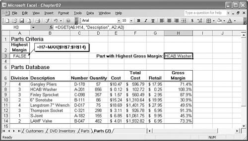

The range $H$7:$H$14 is the Gross Margin field. (Note the use of absolute references.) Excel matches only the record that has the highest gross margin. The DGET() function in cell H3 is straightforward:

 =DGET(A6:H14, "Description", A2:A3)

This formula returns the description of the part that has the highest gross margin.

From Here

If you need more powerful data tools, Microsoft Access should be your Office database program of choice. See Chapter 4, "Taming Access Data."
If you decide to use Access, you can still analyze the data in Excel. In Chapter 6, see the section titled "Analyzing Access Data in Excel."
To learn how to share Excel files with other users, see the section titled "Sharing Excel Workbooks" in Chapter 7.
For information on putting an Excel worksheet on the Web, see the section titled "Publishing an Excel Range, Sheet, or Workbook to the Web" in Chapter 8.
For a few useful Excel VBA macros, see the section "Excel Macros" in Chapter 12.
To learn about workbook protection, see the section "More Options for Protecting Excel Workbooks" in Chapter 14.