Section 4.16. Disk IO Time

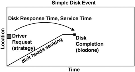
4.16. Disk I/O Time

DTrace makes many I/O details available to us so that we can understand disk behavior. The previous examples measured I/O counts, I/O size, or seek distance, by disk, process, or file name. One measurement we haven't discussed yet is disk response time.

The time consumed responding to a disk event takes into account seek time, rotation time, transfer time, controller time, and bus time, and as such is an excellent metric for disk utilization. It also has a known maximum: 1000 ms per second per disk. The trick is being able to measure it accurately.

We are already familiar with one disk time measurement: iostat's percent busy (%b), which measures disk active time.

Measuring disk I/O time properly for storage arrays has become a complex topic, one that depends on the vendor and the storage array model. To cover each of them is beyond what we have room for here. Some of the following concepts may still apply for storage arrays, but many will need careful consideration.

4.16.1. Simple Disk Event

The time the disk spends satisfying a disk request is often called the service time or the active service time. Ideally, we would be able to read event timestamps from the disk controller itself so that we knew exactly when the heads were seeking, when the sectors were read, and so on. Instead, we have the bdev_strategy and biodone events from the driver presented to DTrace as io:::start and io:::done.

Terminology

We define disk-response-time to describe the time consumed by the disk to service only the event in question. This time starts when the disk begins to service that event, which may mean the heads begin to seek. The time ends when the disk completes the request. The advantage of this measurement is that it provides a known maximum for the disk, 1000 ms of disk response time per second. This helps with the calculation for utilization percentages.

By measuring the time from the strategy (bdev_strategy) to the biodone, we have the driver's view of response time; it's the closest measurement available for the actual disk response time. In reality it includes a little extra time to arbitrate and send the request over the I/O bus, which in comparison to the disk time (which is usually measured in milliseconds) often is negligible. This is illustrated in Figure 4.1 for a simple disk event.

Figure 4.1. Visualizing a Single Disk Event

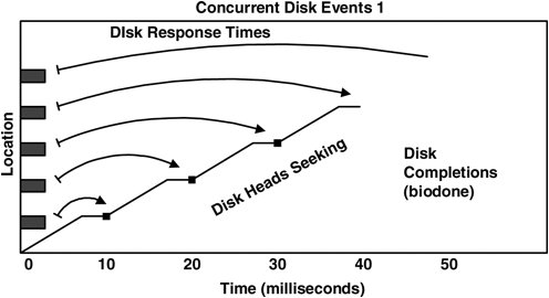
The algorithm to measure disk response time is then

time(disk response) = time(biodone) time(strategy)

We could estimate the total I/O time for a process as a sum of all its disk response times; however, it's not that simple. Modern disks allow multiple events to be sent to the disk, where they are queued. These events can be reordered by the disk so that events can be completed with a minimal sweep of the heads. The following example illustrates the multiple event problem.

4.16.2. Concurrent Disk Events

Let's consider that five concurrent disk requests are sent at time = 0 and that they complete at times = 10, 20, 30, 40, and 50 ms, as is represented in Figure 4.2.

Figure 4.2. Measuring Concurrent Disk Event Times

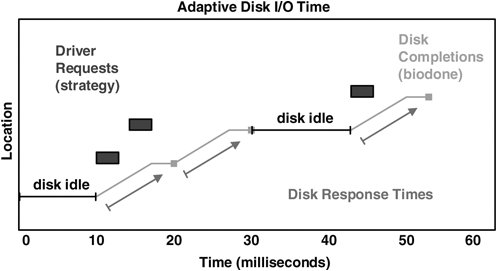
The disk is busy processing these events from time = 0 to 50 ms and so is busy for 50 ms. The previous algorithm gives disk response times of 10, 20, 30, 40, and 50 ms. The total would then be 150 ms, implying that the disk has delivered 150 ms of disk response time in only 50 ms. The problem is that we are overcounting response times; just adding them together assumes that the disk processes events one by one, which is not always the case.

Later in this section we measure actual concurrent disk events by using DTrace and then plot it (see Section 4.17.4), which shows that this scenario does indeed occur.

To improve the algorithm for measuring concurrent events, we could treat the end time of the previous disk event as the start time. Time would then be measured from one biodone to the next. That would work nicely for the previous illustration. It doesn't work if disk events are sparse, such that the previous disk event was followed by a period of idle time. We would need to keep track of when the disk was idle to eliminate that problem.

More scenarios exist, too many to list here, that increase the complexity of our algorithm. To cut to the chase, we end up considering the following adaptive disk I/O time algorithm to be suitable for most situations.

4.16.3. Adaptive Disk I/O Time Algorithm

To cover simple, concurrent, sparse, and other types of events, we need to be a bit creative:

time(disk response) = MIN( time(biodone) time(previous biodone, same dev), time(biodone) time(previous idle -> strategy event, same dev) )

We achieve the tracking of idle -> strategy events by counting pending events and matching on a strategy event when pending == 0. Both previous times above refer to previous times on the same disk device. This covers all scenarios, and is the algorithm currently used by the DTrace tools in the next section.

In Figure 4.3, both concurrent and post-idle events are measured correctly.

Figure 4.3. Best Disk Response Times

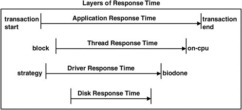
There are some bizarre scenarios for which it could be argued that this algorithm is not perfect and that it is only an approximation. If we keep throwing scenarios at our disk algorithm and are fantastically lucky, we'll end up with an elegant algorithm to cover everything in an obvious way. However, there is a greater chance that we'll end up with an overly complex beastlike monstrosity and several contrived scenarios that still don't fit.

So we consider this algorithm presented as sufficient, as long as we remember that at times it may only be a close approximation.

4.16.4. Other Response Times

Thread-response time is the response time that the requesting thread experiences. This can be measured from the moment that a read/write system call blocks to its completion, assuming the request made it to disk and wasn't cached. This time includes other factors such as the time spent waiting on the run queue to be rescheduled and the time spent checking the page cache if used.

Application-response time is the time for the application to respond to a client event, often transaction oriented. Such a response time helps us understand why an application may respond slowly.

4.16.5. Time by Layer

The relationship between the response times is summarized in Figure 4.4, which depicts a typical sequence of events. This figure highlights both the different layers from which to consider response time and the terminology.

Figure 4.4. Relationship among Response Times

The sequence of events in Figure 4.4 is accurate for raw devices but is less meaningful for block devices. Reads on block devices often trigger read-ahead, which at times drives the disks asynchronously to the application reads; and writes often return from the cache and are later flushed to disk.

To understand the performance effect of response times purely from an application perspective, focus on thread and application response times and treat the disk I/O system as a black box. This leaves application latency as the most useful measurement, as discussed in Section 5.3.