Section 17.4. Chart Types | Excel 2007[c] The Missing Manual

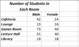
17.4. Chart Types

Although there's a lot to be said for simple column chartsthey can illuminate trends in almost any spreadsheetthere's nothing quite as impressive as successfully pulling off the exotic bubble chart. This section covers the wide range of charts that Excel offers. If you can use these specialized chart types when they make sense, you can convey more information and make your point more effectively.

Note: The following sections explain all of the Excel chart types. To experiment on your own, try out the downloadable examples, which you can find on the "Missing CD" page at www.missingmanuals.com. The examples include worksheets that show most chart types. Remember, to change a chart from one type to another, just select it, and then make a new choice from the ribbon's Insert

Charts section, or use the Chart Tools Design

Type

Change Chart Type command.

17.4.1. Column

By now, column charts probably seem like old hat. But column charts actually come in several different variations (technically known as subtypes ). The main difference between the basic column chart and these subtypes is how they deal with data tables that have multiple series. The quickest way to understand the difference is to look at Figure 17-15, which shows a sample table of data, and Figure 17-16, which charts it using several different types of column charts.

Figure 17-15. This simple table of data records the number of female and male students in several rooms at a university. The category is the room name , and there are two data series: the numbers of male students, and the numbers of female students. This data is perfect for a column chart, but different subtypes emphasize different aspects of the data, as you can see in Figure 17-16.

Note: In order to learn about a chart subtype, you need to know its name. The name appears when you hover over the subtype thumbnail, either in the Insert

Charts list (Figure 17-2) or the Insert Chart dialog box (Figure 17-3).

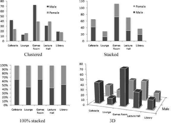
Figure 17-16. The Clustered Column makes it easy to compare the gender of students in each room, but makes it somewhat more difficult to compare different rooms. The Stacked Column is an elegant way to compress the data, and it lets you compare the total number of students in each room without losing the gender information. The 100% Stacked Column makes each column the same height, so it's useless for comparing total student numbers but perfect for comparing how the gender breakup varies depending on the room. (Notice the scale also changes to reflect that you're comparing percentage values.) Finally, the 3-D chart shows you all the data at once by placing the male student counts in front of the female student counts.

100% Stacked Column . The 100% stacked column is like a stacked column in that it uses a single bar for each category, and subdivides that bar to show the proportion from each series. The difference is that a stacked column always stretches to fill the full height of the chart. That means stacked columns are designed to focus exclusively on the percentage distribution of results, not the total numbers.

3-D Clustered Column, Stacked Column in 3-D, and 100% Stacked Column in 3-D . Excel's got a 3-D version for each of the three basic types of column charts, including clustered, stacked, and 100 percent stacked. The only difference between the 3-D versions and the plain- vanilla column charts is that the 3-D charts are drawn with a three-dimensional special effect, that's either cool or distracting, depending on your perspective.

3-D Column . While all the other 3-D column charts simply use a 3-D effect for added pizzazz, this true 3-D column chart actually uses the third dimension by placing each new series behind the previous series. That means if you have three series, you end up with three layers in your chart. Assuming the chart is tilted just right, you can see all these layers at once, although it's possible that some bars may become obscured, particularly if you have several series.

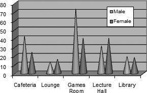
Along with the familiar column and three-dimensional column charts, Excel also provides a few more exotic versions that use cylinders , cones, and pyramids instead of ordinary rectangles. Other than their different shapes , these chart types work just like regular column charts. As with column and bar charts, you can specify how cylinder, cone, and pyramid charts should deal with multiple series. Your options include clustering, stacking, 100% stacking, and layering (true 3-D). See Figure 17-17 for an example.

Figure 17-17. Though a cone chart looks a little different, it's really just a column chart in disguise.

17.4.2. Bar

The venerable bar chart is the oldest form of data presentation. Invented sometime in the 1700s, it predated the column and pie chart. Bar charts look and behave almost exactly the same as column chartsthe only difference being that their bars stretch horizontally from left to right, unlike columns, which rise from bottom to top.

Excel provides almost the same set of subtypes for bar charts as it does for column charts. The only difference is that there's no true three-dimensional (or layered) bar chart, although there are clustered, stacked, and 100% stacked bar charts with a three-dimensional effect. Some bar charts also use cylinder, cone, and pyramid shapes.

Tip: Many people use bar charts because they leave more room for category labels. If you have too many columns in a column chart, Excel has a hard time fitting all the column labels into the available space.

17.4.3. Line

People almost always use line charts to show changes over time. Line charts emphasize trends by connecting each point in a series with a line. The category axis represents a time scale or a set of regularly spaced labels.

Tip: If you need to draw smooth trendlines, you don't want to use a line chart. That's because a line chart connects every point exactly, leading to jagged zigzagging lines. Instead, use a scatter chart (Section 17.4.6) without a line, and add one or more trendlines afterward, as explained in the next chapter (Section 18.5.2).

Excel provides several subtypes for line charts:

Line . The classic line chart, which draws a line connecting all the points in the series. The individual points aren't highlighted.

Stacked Line . In a stacked line chart, Excel displays the first series just as it would in the normal line chart, but the second line consists of the values of the first and second series added together. If you have a third series, it displays the total values of the first three series, and so on. People sometimes use stacked line charts to track things like a company's cumulative sales (across several different departments or product lines), as Figure 17-18, bottom, demonstrates . (Stacked area charts are another alternative, as shown in Figure 17-20.) Stacked line charts aren't as common as stacked bar and column charts.

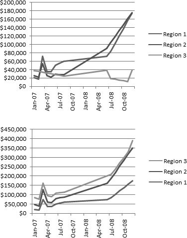
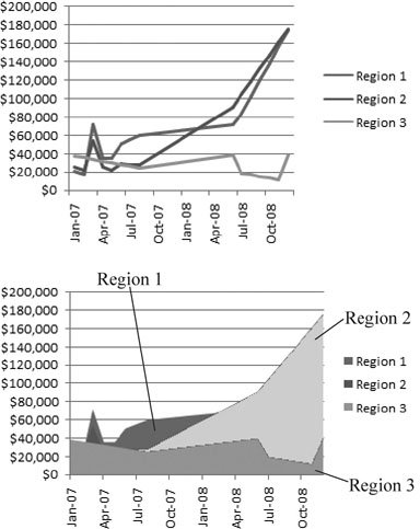
Figure 17-18. Here are two different line chart variationsboth of which show the same information, although you'd never be able to tell that from looking at them quickly.
Top: This chart is a regular line chart that compares the sales for three different regions over time.
Bottom: This chart is a stacked line chart, which plots each subsequent line by adding the numbers from the earlier lines. That makes the stacked line chart a great vehicle for illustrating cumulative totals. For example, sales in Region 3 for April of 2007 appear to top $150,000. That's because the Region 3 line is stacked. It shows a total made up from three components $72,000 (Region 1), $54,000 (Region 2), and $34,300 (Region 3). In this example, the stacked line chart clearly shows that sales spiked early on, but have risen overall, which isn't clear in the top chart. However, the stacked line chart also obscures the differences between the regions. You'd never guess that Region 3 is the underperforming region because this chart reflects the total of all three regions.

Note: Lines can never cross in a stacked line chart because each series is added to the one (or ones) before it. You can change which line is stacked at the top by changing the order of the series. To do this, either rearrange your table of data on the worksheet (Excel places the rightmost column on top) or refer to Section 17.3.6, which describes how you can change the order of your series manually.

100% Stacked Line . A 100% stacked line chart works the same as a stacked line chart in that it adds the value of each series to the values of all the preceding series. The difference is that the last series always becomes a straight line across the top, and the other lines are scaled accordingly so that they show percentages. The 100% stacked line chart is rarely useful, but if you do use it, you'll probably want to put totals in the last series.
Line with Markers, Stacked Line with Markers , and 100% Stacked Line with Markers . These subtypes are the same as the three previous line chart subtypes, except they add markers (squares, triangles , and so on) to highlight each data point in the series.
3-D Line . This option draws ordinary lines without markers but adds a little thickness to each line with a 3-D effect.

17.4.4. Pie

Pie charts show the breakdown of a series proportionally, using "slices" of a circle. Pie charts are one of the simplest types of charts, and one of the most recognizable.

Here are the pie chart subtypes you can choose from:

Pie . The basic pie chart everyone knows and loves, which shows the breakup of a single series of data.
Exploded Pie . The name sounds like a Vaudeville gag, but the exploded pie chart simply separates each piece of a pie with a small amount of white space. Usually, Excel charting mavens prefer to explode just a single slice of a pie for emphasis. This technique uses the ordinary pie subtype, as explained in the next chapter.
Pie of Pie . With this subtype, you can break out one slice of a pie into its own, smaller pie (which is itself broken down into slices). This chart is great for emphasizing specific data; it's demonstrated in the next chapter.
Bar of Pie . The bar of pie subtype is almost the same as the pie of pie subtype. The only difference is that the breakup of the combined slice is shown in a separate stacked bar, instead of a separate pie.
Pie in 3-D and Exploded Pie in 3-D . This option is the pie and exploded pie types in three dimensions, tilted slightly away from the viewer for a more dramatic appearance. The differences are purely cosmetic.

Note: Pie charts can show only one series of data. If you create a pie chart for a table that has multiple data series, you'll see just the information from the first series. The only solution is to create separate pie charts for each series (or try a more advanced chart type, like a donut, which is covered in Section 17.4.10).

17.4.5. Area

An area chart is very similar to a line chart. The difference is that the space between the line and the bottom (category) axis is completely filled in. Because of this difference, the area chart tends to emphasize the sheer magnitude of values rather than their change over time. Figure 17-19 demonstrates.

Area charts exist in all the same flavors as line charts, including stacked and 100% stacked. You can also use subtypes that have a 3-D effect, or you can create a true 3-D chart that layers the series behind one another.

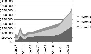
Figure 17-19. This example compares a traditional line chart (top) against the area chart (bottom). As you can see, the area chart makes a more dramatic point about the rising sales in region 2. However, it also obscures the results in region 1.

Tip: Stacked area charts make a lot of sense. In fact, they're easier to interpret than stacked line charts because you can easily get a feeling for how much contribution each series makes to the total by judging the thickness of the area. If you're not convinced, compare the stacked charts in Figure 17-18 (bottom) and Figure 17-20. In the area chart, it's much clearer that region 3 is making a fairly trivial contribution to the overall total.

Figure 17-20. You can create an area chart that doesn't obscure any data, but it needs to be a stacked (as shown here) or 3-D area chart. The stacked area chart shows the combined total of all regions, but it still lets you pick out the most important series. For example, it's clear that Region 3 (the narrow sliver on top of the stack) contributes relatively little to the total, while Region 1 and Region 2 are more important.

17.4.6. XY (Scatter)

XY Scatter charts show the relationship between two different sets of numbers. Scatter charts are common in scientific, medical, and statistical spreadsheets. They're particularly useful when you don't want to connect every dot with a straight line. Instead, scatter charts let you use a smooth "best fit" trendline, or omit the line altogether. If you plot multiple series, the chart uses a different symbol (like squares, triangles, and circles) for each series, ensuring that you can tell the difference between the points.

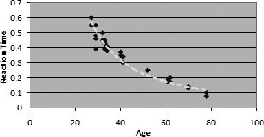
Why would you want to plot data points without drawing a line? For one thing, you may need to draw conclusions from an inexact or incomplete set of scientific or statistical data. Scientific types may use a scatter chart to determine the relationship between a person's age and his reflex reaction time. However, no matter how disciplined the experimenters, they can't test every different age. In addition, their data will include natural variations from the overall trend. (In other words, if the trend is for older people to have gradually slowing reactions , you're still likely to run across a few exceptionally speedy older folks.) In this case, the best approach is to include no line, or use a smooth "best fit" line that indicates the overall trend, as shown in Figure 17-21.

Figure 17-21. This XY Scatter chart shows the relationship between a person's age and his reflex reaction time.

Excel offers several scatter chart subtypes, including:

Scatter with Only Markers . This scatter chart uses data markers to show where each value falls . It adds no lines.
Scatter with Smooth Lines and Markers . This scatter chart adds a smooth line that connects all the data points. However, the points are connected in the order they occur in the chart, which isn't necessarily the correct order. You're better off adding a trendline to your chart, as explained in the next chapter.
Scatter with Straight Lines and Markers . This subtype is similar to the scatter chart with smoothed lines, except it draws lines straight from one point to the next. A line chart works like this, and this subtype makes sense only if you have your values in a set order (from lowest to largest or from the earliest date to the latest).
Scatter with Smooth Lines and Scatter with Straight Lines . These subtypes are identical to the scatter with smooth lines and markers and the scatter with straight lines and markers. The only difference is they don't show data markers for each point. Instead, all you see is the line.

17.4.7. Stock

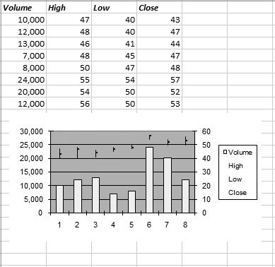
A stock chart displays specialized charts for stocks. Usually, these charts show how a stock value changes over a series of days. The twist is that the chart can display information about the daytime high and the daytime low of the stock, along with its opening and closing value. Excel uses all this information to draw a vertical bar from the stock's low point to its high point on a given day. If you're really ambitious, you can even add volume information (which records the number of shares traded on a given day).

Stock charts are more rigid than most other chart types. In order to use a stock chart, you need to create a column of numbers for each required value. The type of columns you need and their order depends on the stock chart subtype that you select. Here are your choices:

High-Low-Close
Open -High-Low-Close
Volume-High-Low-Close
Volume-Open-High-Low-Close

In each case, the order of terms indicates the order of columns you should use in your chart. If you select Volume-High-Low-Close, then the leftmost column should contain the volume information, followed by another column with the stock's daytime high, and so on. (Technically, you can use the Chart Tools Design Data Select Data command to specify each series, even if its not in the place Excel expects it to be. However, this maneuver is tricky to get right, so it's easiest to just follow the order indicated by the chart type name.) No matter which subtype you use, a stock chart shows only values for a single stock.

Tip: The simplest stock chart (High-Low-Close) is also occasionally useful for charting variances in scientific experiments or statistical studies. You could use a stock chart to show high and low temperature readings . Of course, you still need to follow the rigid stock chart format when ordering your columns.

Figure 17-22 shows an example of a Volume-High-Low-Close.

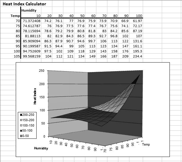
17.4.8. Surface

A surface chart shows a 3-D surface that looks a little like a topographic map, complete with hills and valleys. Surface charts are different from most other charts in that they show the relationship of three values. Two category axes (X and Y) determine a data point's position. The value determines the height of the data point (technically known as the Z-axis). All the points are linked to create a surface.

Surface charts are neat to look at, but ordinary people almost never create them as they're definitely overkill for tracking your weekly workout sessions. For one thing, to make a good surface chart, you need a lot of data. (The more points you have, the smoother the surface becomes.) Your data points also need to have a clear relationship with both the X and Y axes (or the surface you create is just a meaningless jumble ). Usually, rocket-scientist types use surface charts for highly abstract mathematical and statistical applications. Figure 17-23 shows an example.

Figure 17-22. The Volume-High-Low-Close chart shows a combination of related information. The columns at the bottom show the number of shares traded (using the value scale on the left). The lines above these columns show the stock price (using the value scale on the right). For each day, a bar that spans from the day's low to the day's high represents the stock price. The closing price is marked with a tick in the middle of the bar. If you like, you can add a trendline to show the movement of the stock price using the techniques explained in the next chapter.

Figure 17-23. A surface chart usually represents scientific data or mathematical models. Here, the surface chart represents a heat index table. Heat index tables show the perceived temperature under different conditions of humidity. If it's 70 degrees with 90 percent humidity, the dampness makes it feel like 66.9. On the other hand, if it's 85 with 90 percent humidity, it feels to a human observer like a balmy 102.

17.4.9. Donut

The donut chart (Figure 17-24) is actually an advanced variation on that other classic food-themed chart, the pie chart. But while a pie chart can accommodate only one series of data, the donut can hold as many series as you want. Each series is contained in a separate ring. The rings are one inside the other, so they all fit into a single compact circle.

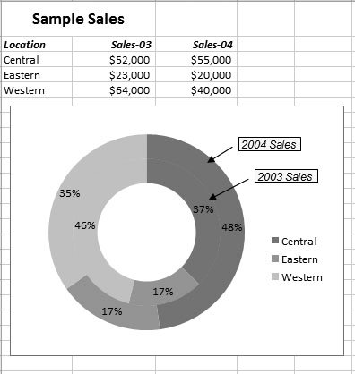
Figure 17-24. Here, a donut chart compares the sales in two different years . The inner ring shows the sales for 2003, broken down by region. The outer ring shows the sales for 2004. Donut charts sometimes need a bit of customizing before they look right. Here, the chart has labels that detail the percentage of each slice, and the year represented by each ring. (You can learn how to add these labels using Excel's drawing tools in Chapter 19.)

The donut chart's ideal for comparing the breakdown of two different sets of data. However, the data on the outside ring tends to become emphasized , so make sure this series is the most important. To change the order of the series, see Section 17.3.6.

Donuts have two subtypes: standard and exploded. (An exploded donut doesn't suggest a guilty snack that's met an untimely demise. Instead, it's a donut chart where the pieces in the topmost ring are slightly separated.)

Although the donut chart can hold as many series as you want, if you add more than two or three, the chart may appear overly complicated. No matter what you do, the center of the donut never gets filled in (unless you decide to add some text there using Excel's drawing tools, which are covered in Chapter 19).

Tip: Think twice before you use a donut chart in a presentation. Most Excel gurus avoid this chart because it's notoriously difficult to explain.

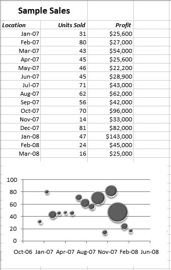
17.4.10. Bubble

The bubble chart is an innovative variation on the scatter chart. It plots only a single series, and it never draws a line. Each point is marked with a circleeither an ordinary circle or a three-dimensional sphere, depending on the subtype you choose. The extra frill is that the bubble sizes change based on a second set of related values. The larger the value, the larger the data point bubble. In any bubble chart, the largest bubble is always the same size . Excel scales the other bubbles down accordingly. Figure 17-25 shows an example.

Figure 17-25. Each bubble's position represents two values: the month (the category axis) and the number of units sold (the value axis). Each bubble's size reflects the profit generated by the units sold.

17.4.11. Radar

The radar chart (Figure 17-26) is a true oddity, and it's typically used only in specialized statistical applications. In a radar chart, each category becomes a spoke, and every spoke radiates out from a center point. Each series has one point on each spoke, and a line connects all the points in the series, forming a closed shape. All these spokes and lines make the chart look something like the radar on an old-time submarine .

You have three radar subtypes: the standard radar chart; a radar chart with data markers indicating each point; and a filled radar, where each series appears as a filled shape, somewhat like an area chart. No matter what subtype you use, choosing data for a radar chart isn't easy.

Figure 17-26. This filled radar chart compares the products sold in sales offices in two different cities. Because all the categories (in this case, the various products) are joined into a closed shape, the radar chart acts somewhat like an area chart, so you can judge the significance of values by looking at the size and shape of the area. It's easy to see that bicycles are selling well with customers in the New York store, while trucks lead the way in Paris. If the two series had similar results, you couldn't effectively use a filled radar chart, because some of the data would be obscured.