Section 10.3. Depreciation | Excel 2007[c] The Missing Manual

10.3. Depreciation

Another common calculation in the world of finance is depreciation . Simply stated, depreciation is how much the value of an asset decreases over time. All assets that depreciate begin with a certain value (which you determine) and then depreciate over the course of a lifetime (which you specify). At the end of an asset's life, from an accounting perspective, the asset is deemed to be useless and without value.

POWER USERS' CLINIC
A Better NPV( )

Excel also provides versions of NPV( ) and IRR( ) that don't assume that payments are made (or profits realized) on fixed dates, once per period. These functions are XIRR( ) and XNPV( ). Using them's a little bit more complicated because you need to supply not only the cash flows, but also the corresponding dates when each transaction occurs. You do this by submitting two cell ranges: the first range has the cash flows, and the second range has the dates.

 XNPV(rate, cashflow_range, date_range) XIRR(cashflow_range, date_range)

The two ranges must be exactly the same size (that is, they must include the same number of cells ), and must line up logically. In other words, Excel assumes that the first cash flow in the cash flow range is deposited on the first date in the date range.

Excel offers four basic depreciation functions (explained below), which can help you determine how much value your asset has lost at any given point in time. You'll use these values if you want to sell the asset, or if you're attempting to calculate the current net worth of a business. Depreciation can also figure into tax calculations and business losses; a company could write off a loss based on the value an asset has lost.

Note: The depreciation of an asset isn't as straightforward as interest calculations. You use a certain amount of guesswork when you're deciding what an asset is worth and how rapidly its value declines. An asset can include almost anything, from a piece of equipment or property to a patented technology. It may depreciate due to wear and tear, obsolescence, or market conditions (like decreased demand and increased supply).

In order to assign a value to a depreciated asset, Excel makes a logical guess about the way in which the asset's depreciating. You can use any of a number of accepted ways to make this guess (or estimate, as financial types prefer to call it). The easiest way of depreciating an asset is the straight-line depreciation method, where the value of the asset decreases regularly from the starting value to the final value. However, this approach isn't necessarily realistic for all assets.

Excel supports four basic depreciation functions, each of which figures depreciation in a slightly different way:

SLN( ) . SLN( ) uses simple straight-line depreciation, where the cost of the asset minus its scrap value (the value of the asset if sold purely as raw material) is simply divided by the life span of the asset. In other words, if the life span's 10 years , the book value of the asset is depreciated by 10 percent of the original value each year. SLN( ) is the only form of depreciation that proceeds regularly. All other types of depreciation are known as accelerated depreciation functions because they assume that the asset's greatest loss in value occurs early on, rather than evenly over several years. As a result, these accelerated depreciation functions are often more realistic.
SYD( ) . SYD( ) uses the sum-of-years-digits depreciation method. This method starts with a larger depreciation rate, which is gradually lowered as the asset becomes less valuable . SYD( ) is a good all-around choice for most depreciation calculations.
DDB( ) . DDB ( ) uses the double declining balance depreciation method, which is like straight-line depreciation on steroids. It reduces an asset by double the percentage of the SLN( ) method, which makes for a fast reduction in value (and a hefty tax write-off). In other words, if the life span is 10 years, the book value of the asset is depreciated by 20 percent of the original value each year.

Note: This approach has a problem, however: Eventually the asset will dip below its final value (and even become a negative number). Accountants handle this problem by imposing an additional rule. As soon as the amount of depreciation in any given year is less than the straight-line depreciation amount, you must immediately abandon the DDB( ) method and start calculating depreciation with SLN( ). But it's still up to you to be aware of this and check for this condition. If this sounds messywell, it is.
DB( ) . DB( ) uses the declining balance method, where an asset declines in value by a fixed percentage of its book value every year. Like the SYD( ) and the DDB( ) approaches, this method is an accelerated depreciation function. However, it has a different limitation: You can't specify the final value the asset should have after its lifetime's over (the salvage value).

These functions work with more of less the same arguments, but they produce different results. Here's a look at the syntax of all four functions:

 SLN(cost, salvage, life) SYD(cost, salvage, life, period) DB(cost, salvage, life, period, [month]) DDB(cost, salvage, life, period, [factor])

The cost is the initial value of the asset.
The salvage argument is the value of the asset at the end of its depreciation. If it's lost all value, this is 0.
The life is the number of periods over which the asset is depreciating. It's also known as the useful life of the asset.
The period is a number that indicates the period in which you want to calculate depreciation; it must use the same unit as the life. If you're depreciating an asset over three years, a period of 3 will get you the amount of money that the asset depreciated in the third year. The SLN( ) function doesn't require a period argument because depreciation is the same in every period.
The month is an optional argument supported by the DB( ) function. It specifies the number of months that the asset's in use for the first year. If you leave this out, then Excel assumes 12 months of service.
The factor is an optional argument supported by the DDB( ) function. You multiply the factor by the expected straight-line depreciation to get the actual depreciation. If you omit this argument, then Excel assumes a value of 2 (which is why it's known as double declining depreciation).

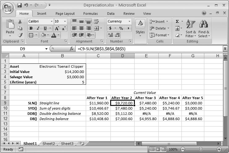
As an example, imagine a company purchases a top-of-the-line computer for $10,000. The computer has a salvage value of $200 after its useful life of five years. To compute its second-year depreciation using the popular SYD( ) method, you'd use the following calculation:

 =SYD(10000, 200, 5, 2)

This calculation indicates that the computer loses $2,613.33 of its value in the second year. However, to calculate the total depreciation so far, you need to add the depreciation in both the first and second year, and subtract that from the initial value, as shown here:

 =10000-SYD(10000, 200, 5, 1)-SYD(10000, 200, 5, 2)

This formula takes the $10,000 total, and subtracts the first- and second-year depreciation ($3,266.67 and $2,613.33, respectively), which gives you a current value of $4,120. You'll notice that with the SYD( ) function, most of the depreciation takes place in the first year, and then each following year the asset loses a smaller amount of its value.

The easiest way to see depreciation at work is to build a worksheet that compares these four different functions. Figure 10-5 shows an example.

Figure 10-5. This worksheet shows depreciation on a sample investment. Once you set the initial value, lifetime value, and salvage value, you can calculate the depreciation. But as you can see, some methods produce faster depreciation than others.

In Figure 10-5, the straight line depreciation is the slowest of all, which makes it less realistic for dealing with the plummeting values of aging high-tech parts . The sum-of-years-digits depreciation provides faster depreciation, yet still ends up with the desired salvage value of $3,000. The last two methods are a little trickier. You can use the double-declining balance approach only for the first two years. In the third year, the depreciation it calculates ($2,044.8) is less than the sum-of-years depreciation value ($2,240), so it's time to switch methods. To underscore that fact, the following cells display the #N/A code. The declining-balance approach works well initially, but then tops out in the last year. Probably, you'll ignore the last calculated value and just use the salvage value of $3,000.

Note: When using double-declining balance depreciation, it's up to you to spot when the method no longer applies. Excel doesn't tell you; instead, it cheerily continues calculating depreciation values, even if the depreciation exceeds the total value of the asset. In Figure 10-5, the #N/A values were typed in by hand.