Section 8.3. Copying Formulas
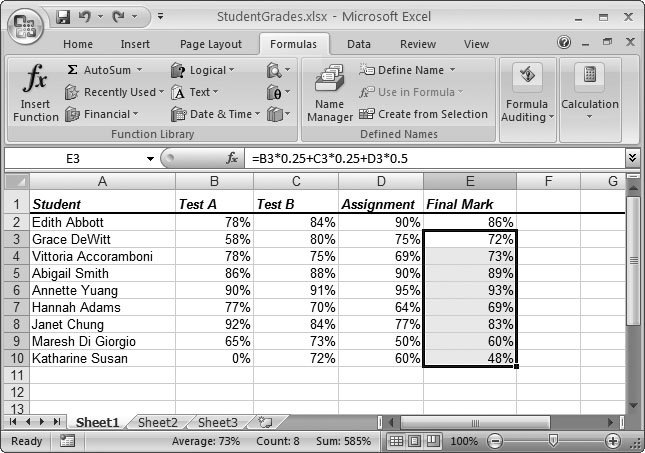
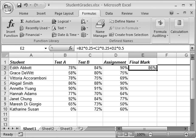
8.3. Copying FormulasSometimes you need to perform similar calculations in different cells throughout a worksheet. For example, say you want to calculate sales tax on each item in a product catalog, the monthly sales in each store of a company, or the final grade for each student in a class. In this section, you'll learn how Excel makes it easy with relative cell references . Relative cell references are cell references that Excel updates automatically when you copy them from one cell into another. They're the standard kind of references that Excel uses (as opposed to absolute cell references, which are covered in the next section). In fact, all the references you've used so far have been relative references, but you haven't yet seen how they work with copy-and-paste operations. Consider the worksheet shown in Figure 8-11, which contains a teacher's grade book. In this example, each student has three grades: two tests and one assignment. A student's final grade is based on the following percentages: 25 percent for each of the two tests, and 50 percent for the assignment.
The following formula calculates the final grade for the first student (Edith Abbott): =B2*25% + C2*25% + D2*50% The formula that calculates the final mark for the second student (Grace DeWitt) is almost identical. The only change is that all the cell references are offset by one row, so that B2 becomes B3, C2 becomes C3, and D2 becomes D3: =B3*25% + C3*25% + D3*50% You may get fed-up entering all these formulas by hand. A far easier approach is to copy the formula from one cell to another. Here's how:
Tip: There's an even quicker way to copy a formula to multiple cells by using the AutoFill feature introduced in Chapter 2 (Section 2.2.3). In the student grade example, you'd start by moving to cell E2, which contains the original formula. Then, you'd click the small square at the bottom-right corner of the cell outline, and drag the outline down until it covers all cells from E3 to E10. When you release the mouse button, Excel inserts the formula copies in the AutoFill region. 8.3.1. Absolute Cell ReferencesRelative references are a true convenience since they let you create formula copies that don't need the slightest bit of editing. But you've probably already realized that relative references don't always work. For example, what if you have a value in a specific cell that you want to use in multiple calculations? You may have a currency conversion ratio that you want to use in a list of expenses. Each item in the list needs to use the same cell to perform the conversion correctly. But if you make copies of the formula using relative cell references, then you'll find that Excel adjusts this reference automatically and the formula ends up referring to the wrong cell (and therefore the wrong conversion value).
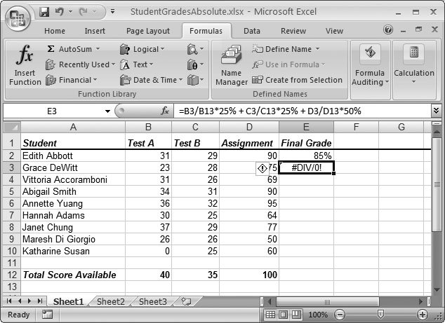
Figure 8-13 illustrates the problem with the worksheet of student grades. In this example, the test and assignment scores aren't all graded out of 100 possible points; each item has a different total score available (listed in row 12). In order to calculate the percentage a student earned on a test, you need to divide the test score by the total score available. This formula, for example, calculates the percentage for Edith Abbott's performance on Test B: =B2/B12*100% To calculate Edith's final grade for the class, you'd use the following formula: =B2/B12*25% + C2/C12*25% + D2/D12*50% Like many formulas, this one contains a mix of cells that should be relative (the individual scores in cells B2, C2, and D2) and those that should be absolute (the possible totals in cell B12, C12, and D12). As you copy this formula to subsequent rows, Excel incorrectly changes all the cell references, causing a calculation error. Fortunately, Excel provides a perfect solution. It lets you use absolute cell references cell references that always refer to the same cell. When you create a copy of a formula that contains an absolute cell reference, Excel doesn't change the reference (as it does when you use relative cell references; see the previous section). To indicate that a cell reference is absolute, use the dollar sign ($) character. For example, to change B12 into an absolute reference, you would add the $ character twice, once in front of the column and once in front of the row, which changes it to $B$12.
Here's the corrected class grade formula (for Edith) using absolute cell references: =B2/$B*25% + C2/$C*25% + D2/$D*50% This formula still produces the same result for the first student. However, you can now copy it correctly for use with the other students. To copy this formula into all the cells in column E, use the same procedure described in the previous section on relative cell references. 8.3.2. Partially Fixed ReferencesYou might wonder why you need to use the $ character twice in an absolute reference (before the column letter and the row number). The reason is that Excel lets you create partially fixed references. To understand partially fixed references, it helps to remember that every cell reference consists of a column letter and a row number. With a partial fixed reference, Excel updates one component (say, the column part) but not the other (the row) when you copy the formula. If this sounds complex (or a little bizarre), consider a few examples:
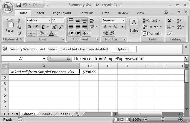
Tip: You can quickly change formula references into absolute or partially fixed references. Just put the cell into edit mode (by double-clicking it or pressing F2). Then, move through the formula until you've highlighted the appropriate cell reference. Now, press F4 to change the cell reference. Each time you press F4, the reference changes. If the reference is A1, for instance, it becomes $A$1, then A$1, then $A1, and then A1 again. 8.3.3. Referring to Other Worksheets and WorkbooksMost formulas refer to the cells in a single worksheet. Excel does, however, let you use formulas that refer to cells in other worksheets or even other files. To reference a cell in another worksheet, you simply need to preface the cell with the worksheet name , followed by an exclamation mark. For example, say you've created a formula to double the value of the number in cell A1 on a worksheet named Sheet1. You'd use this formula: =A1*2 If you want to use the same formula in another worksheet (in the same workbook), you'd insert this formula in the new worksheet: =Sheet1!A1*2 Note: If you use the point-and-click method to build formulas, you'll find that you don't need to worry about the syntax for referring to cells on other worksheets. If you switch to another worksheet while you're building a formula, Excel automatically inserts the correct reference to the worksheet name. It's fairly common for one worksheet to reference another within the same workbook file. (For a refresher on the difference between worksheets and workbooks see Section 4.1.) in Section 9.1.1, you'll see an example where one worksheet includes a product catalog, and a second worksheet builds an invoice. In that example, the second worksheet uses formulas that refer to data on the first sheet. It's less common for a worksheet to refer to data in another file . The potential problem with this type of link is that there's no way to guarantee that referenced files will always be available. If you rename the file or move it to a different folder, then the link breaks. Fortunately, Excel doesn't leave you completely stranded in this situationinstead, it continues with the most recent version of the data it was able to retrieve. You can also tweak the link to point to the new location of the file. To create a link to a cell in another workbook, you need to put the file name at the beginning of the reference and then enclose it in square brackets. You follow the file name with the sheet name, an exclamation mark, and the cell address. Here's an example: =[SimpleExpenses.xlsx]Sheet1!B3 If the file name or the sheet name contains any spaces, you need to enclose the whole initial portion inside apostrophes , like so: ='[Simple Expenses.xlsx]Sheet1'!B3 When you enter this formula, Excel checks to see if this file is already open in another Excel window. If not, then Excel attempts to find the file in the current folder (that is, the same folder that holds the workbook you're editing). If it can't find the file, it shows a standard Open dialog box. You can use this dialog box to browse to the file you want to use. Once you select the file, Excel updates the formula accordingly . Excel performs a little sleight of hand with formulas that reference other files. If the referenced workbook's currently open, the formula displays only the file name. However, once you close the referenced file, the formula changes so that it includes the full folder path . Excel makes this change automatically, whether you type a file name in by hand or build the formula by pointing and clicking on cells in another open workbook. Here's an example of what the full formula looks like when you close the file that contains the Sheet1 worksheet (split over two lines to fit the page): ='[C:\Documents and Settings\Matthew\My Documents\Simple Expenses.xlsx]Sheet1'!B3 8.3.3.1. Updating formulas that refer to other workbooksYou use a formula that refers to another workbook (rather than just copying the information you need) when you know the information in that workbook might change. So what does Excel do to keep your linked information up to date? It all depends. If the linked workbook is currently open, Excel spots any changes right away. For example, imagine you have a workbook named Summary.xlsx that refers to cell B3 in a workbook named SimpleExpenses.xlsx (as shown in the previous example). When you modify the number in B3 in SimpleExpenses.xlsx, Excel recalculates the linked formula in Summary.xlsx immediately. It's a different story if you work with both files separately . For example, imagine you close Summary.xlsx, change the total in SimpleExpenses.xlsx, and then close SimpleExpenses.xlsx. The next time you open Summary.xlsx, Excel is in a difficult position. It needs to get the updated information in SimpleExpenses.xlsx, but it doesn't want to open the file to do so (at least not without your OK). So instead, the Summary.xlsx file uses the most recent informationthe value it pulled out of cell B3 the last time SimpleExpenses.xlsx was open. Excel also shows a message bar just above the grid of cells, warning you that it hasn't retrieved the latest information (Figure 8-14).
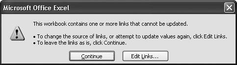
If you want to update your linked formulas, click the message bar's Options button (shown in Figure 8-14). When the Security Options dialog box appears, choose "Enable this content", and then click OK. Excel opens the linked workbook (in this case, SimpleExpenses.xlsx) behind the scenes, and then uses the latest information to recalculate your formula. Tip: You need to click the Options button, and then turn on your links every time you open a workbook like Summary.xlsx. If you get tired of this process, then you may be interested in creating a trusted location a folder on your hard drive where you can store your workbooks so Excel knows they're kosher. When you use a trusted location, Excel doesn't give you a security warninginstead, it refreshes your linked formulas automatically. Section 27.3.2 shows how to set up a trusted location. Sometimes, despite the best of intentions, your formula points to a workbook that Excel can't find. For example, if you rename SimpleExpenses.xlsx or move it to another folder, then you'll run into this problem. In this situation, Excel gives you an error message when you attempt to switch on your links (Figure 8-15).
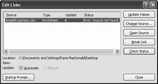
If you know that a link's gone bad, you've got a problemdepending on how many linked formulas your workbook has, you could be stuck updating dozens of cells. Fortunately, the Edit Links dialog box (shown in Figure 8-16) gives you an easier alternative. Rather than changing each formula by hand, you can "relink" everything by pointing Excel to the right file. The Edit Links dialog box appears automatically when an error occurs, but you don't need to wait for a problem to change a link. You can also get to the Edit Links dialog box on your own by choosing Data
The Edit Links dialog box is invaluable for fixing broken links. In addition, some of the buttons in the Edit Links dialog box work with links that aren't broken. They include:
|
 Clipboard