Section 1.3. Navigating in Excel
1.3. Navigating in ExcelLearning how to move around the Excel grid quickly and confidently is an indispensable skill. To move from cell to cell, you have two basic choices:
As you move from cell to cell, you see the black focus box move to highlight the currently active cell. In some cases, you may want to cover ground a little more quickly. You can use any of the shortcut keys listed in Table 1-1. The most useful shortcut keys include the Home key combinations, which bring you back to the beginning of a row or the top of your worksheet. Note: Shortcut key combinations that use the + sign must be entered together. For example, "Ctrl+Home" means hold down the Ctrl key and press the Home key at the same time. Other key combinations work in sequence. For example, the key combination "End, Home" means press End first, take your finger off it, and then press Home.
Excel also lets you cross great distances in a single bound using a Ctrl+arrow-key combination. These key combinations jump to the edges of your data. Edge cells include cells that are next to other blank cells. For example, if you press Ctrl+ The Ctrl+arrow-key combinations are useful if you have more than one table of data in the same worksheet. For example, imagine you have two tables of data, one at the top of a worksheet and one at the bottom. If you're at the top of the first table, you can use Ctrl+ Tip: You can also scroll anywhere you want in your spreadsheet with the help of the scroll bars at the bottom and on the right side of the worksheet. Finding your way around a worksheet is a fundamental part of mastering Excel. Knowing your way around the larger program window is no less important. The next few sections help you get oriented, pointing out the important stuff and letting you know what you can ignore altogether. 1.3.1. The MenusYou probably think that the classic pull-down menu is the simplest element on your screen. But in Excel 2003, the menus force you to take part in an awkward game of hide-and-seekunless you take a few steps to tame them. Figure 1-7 shows two different versions of the same Tools menu. The first is the "simplified" version Excel shows you automatically. The idea behind the simplified menu is that by hiding some of the more advanced choices, Excel helps you find what you want more quickly. To its credit, Excel goes one step further and actually stores information about what menu options you use. That means that when you select a menu like Tools, you see a simplified version that includes all the choices you typically use. Excel calls this a personalized menu, and the options change as you use the menu. If you can't find an item you're all but certain was in a particular menu, you can temporarily expand the menu to show every option. Simply click the expand icon at the bottom of the personalized menu (it looks like two arrows pointing down). Alternatively, you can just hover over the expand icon with the mouse. Figure 1-7. Top: Personalized menus attempt to make life easier by hiding the options you don't use much. This innovation is often more trouble than it's worth, however, because it's hard to remember how a menu is organized when it's constantly changing. |
 (or Shift+Tab)
 (or Enter)
 to jump to the bottom of the first table, skipping all the rows in between. Press Ctrl+
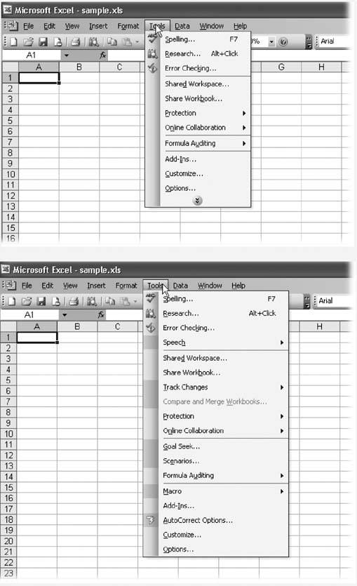
| GEM IN THE ROUGH Getting Somewhere in a Hurry |
If you're fortunate enough to know exactly where you need to go, you can use the Go To feature to make the jump. Go To moves to the cell address that you specify. It's useful in extremely large spreadsheets, where just scrolling through the worksheet takes half a day. To show the Go To dialog box, select Edit 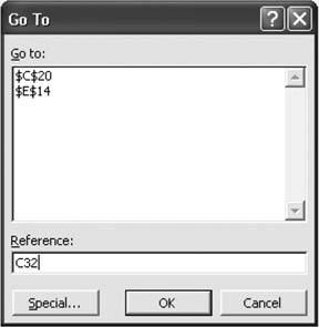 The Go To feature becomes more useful the more you use it. That's because the Go To window maintains a list of the most recent cell addresses that you've entered. In addition, every time you open the Go To window, Excel automatically adds the current cell to the list. This feature makes it easy to jump to a far off cell and quickly return to your starting location by selecting the last entry in the list. In the list, Excel writes cell addresses a little differently than the format you use for typing them in. Namely, dollar signs are added before the row number and column letter. Thus, C32 becomes $C$32, which is simply the convention that Excel uses for fixed cell references. (You learn much more about the different types of cell references in Chapter 7.) |
Note: When you turn off personalized menus in Excel, you're actually changing a setting that affects all Office programs. Thus, you're turning them off in other Office applications on your computer, including Word and Outlook.
1.3.2. The Task Pane
The Task Pane is the hub of activity in Excel. It provides information and controls to let you accomplish a specific task, like searching for help or opening a new spreadsheet. The Task Pane is a genuine improvement over the old way of getting work done in Excel. Instead of forcing you to dig through several different menus, the Task Pane gathers everything you need into one convenient location. It also lets you see your spreadsheet data at all times and continue working with it (Figure 1-8). Other Excel windows aren't nearly as politethey lock you out of your spreadsheet and obscure your data until you're finished with them. For example, if you choose to format a group of cells, you can't edit any information in the Excel grid until you finish using the Format Cells dialog box and click OK.
Unfortunately, the Task Pane lets you perform only a limited number of tasks, so it doesn't replace Excel's menus and toolbars. Still, it's handy. To select the task that you want to perform, click the title of the Task Pane window. Figure 1-8 shows the list of possible tasks. Note that the current task is identified by a check-mark.
Tip: The Task Pane window often uses hyperlinks, which look like ordinary text, but you can click them to trigger an action, just like you click a toolbar button or pick an option from the menu. To find out if a given text item is a hyperlink, hover over it with the mouse. If the text becomes underlined, it's a hyperlink. (Try the "Create a new workbook" link, for example, which you can see at the bottom of Figure 1-8.)
You can close the Task Pane window at any time by clicking the "x" in the top-right corner of the window. Or, you can quickly hide or show the Task Pane by choosing View  Task Pane.
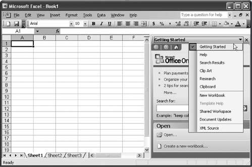
Figure 1-8. When you first start Excel, the Task Pane appears on the right with the Getting Started task displayed. To switch to any of 10 other tasks, click the drop-down arrow in the window title and choose the task from the list.
All the Office programs include a Task Pane, but the list of available tasks differs. In Excel 2003, you can use the following tasks:
Getting Started. This task is the one you see when you first start Excel. It provides a list of links from Microsoft's Office Web site (http://office.microsoft.com). For example, you can click "Get the latest news about using Excel" to open up your Internet browser with a list of bulletins about new developments on Planet Excel. You can also search the Office Web site for help files by using the "Search for" box. Finally, at the bottom of the Getting Started window are a couple of hyperlinks that let you open an existing spreadsheet or create a new one.
Help. This task lets you search the built-in Excel help files. If your computer is connected to the Internet, this search actually branches out to Microsoft's online Excel documentation, where it retrieves the latest relevant information. For more information about getting help in Excel, check out Appendix A.
Search Results. The Search Results task window works in conjunction with the Help or Getting Started tasks. Both of these tasks let you search the online Office help. Once Excel has finished a search, the Search Results task window appears with a list of matching results.
Tip: You can navigate back to the Search Results task window at any time to see the results from your most recent search.
Clip Art. This extremely useful task lets you find clip art using a straightforward keyword search. For example, if you need to impress agricultural clients with a giant farm animal interposed between your columns of numbers, type "sheep" into the Clip Art search. After a short delay, a series of tiny pictures appears. You can then drag these pictures directly onto your spreadsheet and resize them as needed. The Clip Art search can find matching pictures that are installed on your computer (as a part of Office 2003) and free graphics from the Office 2003 Web site.
Research. While the Clip Art task let you find the graphics you need, the Research task lets you find the information you want. This search can include looking a term up in a dictionary or thesaurus, or performing an online search for news articles, stock quotes, encyclopedia entries, and more. Best of all, you perform the search inside Excel, so you can drag and drop results into your worksheet.
Clipboard. Excel lets you place multiple pieces of data on the clipboard at the same time. You can examine these pieces of datawhich may be snippets of text, pictures, charts, or entire cell ranges (groups of cells)using the Clipboard task window. You can then remove items or drag them back onto your spreadsheet, giving you a great way to quickly rearrange your tables. For more information, see Section 3.2.3.
New Workbook. This task lets you create a new spreadsheet. You have the choice of creating a blank spreadsheet or creating a spreadsheet based on a prebuilt template (fully designed spreadsheets that let you plug in numbers and perform specific tasks like figuring out loan payment amounts or creating sales invoices). Chapter 8 is all about templates.
Shared Workspace and Document Updates. These advanced tasks let you manage the way several people can collaborate on a spreadsheet through a shared workspace, although you can't use these features unless you have SharePoint Server (a powerful collaboration tool included with Windows 2003 Server).
XML Source. Excel 2003 introduces a bunch of geek-only features that let spreadsheet wizards import and export XML data, which is a special format used to organize information so that it's more easily exchanged between different operating systems and different programs.
| EXCEL 2002 CORNER The Changing Face of the Task Pane |
The Task Pane is one of the more changeable ingredients in Excel. If you're using Excel 2002, you'll notice that the list of tasks is dramatically shorter, with only four basic tasks:
So what about the missing tasks? A few of themincluding Research, Shared Workspace and Document Updates, and XML Sourcecorrespond to features that Excel 2002 doesn't provide. In other cases, it's just a cosmetic difference. For example, Excel 2002 provides a similar catalog of searchable help, but it doesn't provide a snazzy Help task to help you get to it. Instead, you need to use the ordinary Help menu. |
Note: Occasionally, you come across tasks you can't easily reach from the Task Pane menu. For example, when you launch a file search from the File menu in Excel 2003 (as described at the end of this chapter), the Basic File Search task appears, but it isn't available through the main Task menu. (In contrast, Excel 2002 does offer file searching as one of its Task Pane options.)
1.3.3. The Toolbars
Excel, like any self-respecting Windows program, is filled with toolbars (Figure 1-9). You can think of toolbars as a lighter version of the Task Pane windows. Like the Task Pane, toolbars group together buttons for a common task (like manipulating pictures, creating charts, reviewing a document, and so on). Also like the Task Pane, toolbars stay out of your way while you work. But unlike the Task Pane, toolbars don't provide much information to help you out if you aren't already an expert. You can hover over a toolbar button to see a one- or two-word title for a button (as shown in Figure 1-9), but that's about it.
Figure 1-9. Hovering over a toolbar button displays (very) brief tooltip text that describes that button.
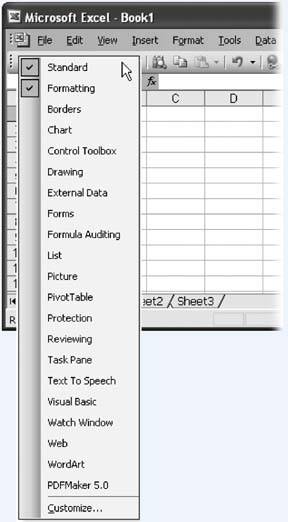
To see a menu that lists all the available Excel toolbars (Figure 1-10), right-click any toolbar, or choose View  Toolbars. The toolbars that have a checkmark next to their name are the ones that are currently visible. You can use this list to show new toolbars (select a toolbar that isnt checked) or hide visible ones (click a checked toolbar).
Figure 1-10. In this picture, only two toolbars are currently displayed: the all-important Standard and Formatting toolbars. To show other toolbars, right-click anywhere on one of the currently displayed toolbars for a menu of toolbar choices, as shown here.
Tip: Resist the urge to display all the toolbars at the same time, or you'll end up with a heavily cluttered window that shmushes your worksheet into a tiny corner.
Excel provides a grand total of 19 toolbars (not including the Task Pane, which is really a completely different type of window). In addition, some third-party products automatically add Excel toolbars to your computer. For example, if you install the full version of Adobe Acrobat (the software for creating PDF files), you find a new PDFMaker toolbar. Excel always shows third-party toolbars at the end of the toolbar list.
Note: To make life a little easier, Excel opens some toolbars automatically when you need them. For example, when you select a chart, the Chart toolbar springs into action at the top of the window, only to disappear again as soon as you select a different part of your spreadsheet. You see the same behavior when you create lists and work with pictures.
Excel starts you off with two important toolbars:
Standard. This toolbar includes the most commonly used buttons, like those for saving, opening, and printing spreadsheets. It also holds buttons for cutting and pasting data, undoing changes, and inserting charts.
Formatting. This toolbar includes buttons for changing text font, alignment, and style. You learn about these options in Chapter 4.
Both of these toolbars use a standard arrangement of buttons that's a close replica of what you've probably seen in other Office programs, like Microsoft Word.
1.3.3.1. Moving toolbars
You can drag toolbars anywhere on the Excel window, which is useful, for instance, if you're looking for ways to maximize the amount of screen space you have. For example, you can drag toolbars above the menu or to the left or right side of the window, in which case they change from a horizontal row of buttons to a vertical column of buttons. You can even drag a toolbar away from the window's edge so that it becomes a standalone, resizable floating window like the one shown in Figure 1-11.
Figure 1-11. You can arrange toolbars in various places in the Excel window.

To move a toolbar, follow these three steps:
Position your mouse over the left edge of the toolbar.
The left edge of the toolbar has a series of dots to show you where the toolbar "grip" is. The mouse pointer changes to a four-way arrow to indicate you're in the right place.
Start dragging the toolbar.
As you move the toolbar, other toolbars automatically rearrange themselves.
Release the mouse when you've got the toolbar where you want it.
Figure 1-11 shows some of the different ways you can position toolbars, and you can always drag toolbars back to their original positions.
Toolbars remember their last position. Thus, if you move a toolbar and then hide it, it appears in its new position the next time you show it. (To show a toolbar, click View Toolbars and turn on the checkbox next to the toolbar you want to show.)
Tip: Sometimes a toolbar inadvertently gets loose from the edge of the window. Fortunately, there's a quick way to return a rogue floating toolbar to its last docked position: just double-click the toolbar's title bar.
1.3.3.2. Toolbars with missing buttons
Depending on the width of your window and the arrangement of your toolbars, some buttons on a toolbar may be invisible. You can tell if some are in hiding by checking out the toolbar's right edge. If you see a symbol that includes two tiny triangles, you know that additional items lurk beneath the surface. To reach these missing buttons, click the right side of the toolbar, which opens a menu with the rest of the buttons.
1.3.3.3. Toolbar tricks
When you click the arrow on the right edge of a toolbar, Excel shows you not only any hidden buttons, but a couple of toolbar options, too. "Add or Remove Buttons" lets you customize the toolbar. You can also choose "Show Buttons on One Row" to put all the buttons from the Standard and Formatting toolbars on one horizontal row at the top of the window. While this arrangement gives you more space for your data, it also hides most of the buttons on your toolbars, which leads to extra clicking around when you need those babies.
Note: If you've chosen "Show Buttons on One Row," the menu item changes to "Show Buttons on Two Rows" (which you can click to pop the Standard and Formatting toolbars back into separate rows).
1.3.4. The Formula Bar
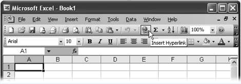
The Formula bar appears above the worksheet grid but below the other Excel toolbars (Figure 1-12). It displays the address of the active cell (like B3) on the left edge, and it also shows you the content of the current cell.
Figure 1-12. The Formula bar shows information about the active cell.
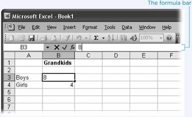
You can use the Formula bar to enter and edit data, instead of editing directly in your worksheet. This approach is particularly useful when a cell contains a formula or a large amount of information, because you have more space to work with in the Formula bar than in a typical cell. Just as with in-cell edits, formula bar edits let you press Enter to confirm your changes or Esc to cancel them. You can also use the mouse: between the cell address and the box showing its contents, click the green checkmark to commit your modification or the red "X" to roll it back.
Note: You can hide (or show) the Formula bar by choosing View
Formula Bar. But its such a basic part of Excel that it would be unwise to get rid of it. Instead, keep it around until Chapter 7, where you see how to build formulas.1.3.5. The Status Bar
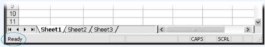
Though people often overlook it, the Status bar (Figure 1-13) is a good way to keep on top of what Excel's currently doing. For example, if you save or print a document, the Status bar, which is located at the bottom of the Excel window, shows the progress of the printing process. If you're performing a quick action, the progress indicator may disappear before you have a chance to even notice it. But if you're performing a time-consuming operationsay, printing out an 87-page table of the airline silverware you happen to ownyou can look to the Status bar to see how things are coming along. (To hide or show the Status bar, choose View Status Bar.)
Figure 1-13. The always-available Status bar displays basic status text (which just says "Ready" in this example) and various indicators when they're active ("CAPS" and "SCRL" in this example).
Usually the Status bar displays one of two things:
The word "Ready." Ready means that Excel isn't doing anything much at the moment, other than waiting for you to take some action.
The word "Edit." Edit means the cell is currently in Edit mode, and pressing the left and right arrow keys moves through the cell data, instead of moving from cell to cell. As you learned on Section 1.2, you can place a cell in edit mode or take it out of edit mode by pressing F2.
In addition, the compartments at the rightmost side of the Status bar give you a few other pieces of information, like whether Caps Lock is turned on. Table 1-2 describes these special values.
INDICATOR | MEANING |
|---|---|
CAPS | Every letter you type in is automatically capitalized. To turn this feature on or off, hit the Caps Lock key on your keyboard. |
NUM | Many people find it fastest to use the numeric keypad (typically at the right side of your keyboard) to type in numbers. When this sign is off, the numeric keypad controls cell navigation instead. To turn this feature on or off, press the Num Lock key. |
SCRL | When this sign is on and you use the arrow keys, the worksheet scrolls as normal, but the active cell doesn't change. This feature lets you look at all the information you have in your worksheet without losing track of the place you're currently in. You can turn this feature on or off by pressing the Scroll Lock key. |
OVR | Overwrite mode is turned on. If you type new characters in edit mode, they overwrite existing characters (rather than displacing them). You can turn this feature on or off by pressing the Insert key. |
END | You have pressed the End key, which is the first key in a two-key combination; the next key determines what happens. For example, hit End and then Home to move to the bottom-right cell in your worksheet. See Table 1-1 for a list of key combinations, some of which use End. |
EXT | As you press the arrow keys, Excel automatically selects all the rows and columns you crossin other words, your selection is extended, which is what the three-letter abbreviation refers to. Extended mode is a useful keyboard alternative to dragging your mouse to select swaths of the grid. To turn this mode on or off, press F8. You can learn more about selecting cells and moving them around in Chapter 3. |
FIX | Indicates that Excel will automatically add a set number of decimal places to the values you enter in any cell. For example, if you set Excel to use two fixed decimal places and you type the number 5 into a cell, Excel actually enters 0.05. This seldom-used featured is handy for speed typists who need to enter reams of data in a fixed format. You can turn this feature on or off by selecting Tools |
Note: You can also use the Status bar to display quick totals as you select groups of numbers. This trick is explained in the box "A Truly Great Calculation Trick" on Section 3.2.
EAN: 2147483647
Pages: 85
- Chapter I e-Search: A Conceptual Framework of Online Consumer Behavior
- Chapter II Information Search on the Internet: A Causal Model
- Chapter III Two Models of Online Patronage: Why Do Consumers Shop on the Internet?
- Chapter X Converting Browsers to Buyers: Key Considerations in Designing Business-to-Consumer Web Sites
- Chapter XVI Turning Web Surfers into Loyal Customers: Cognitive Lock-In Through Interface Design and Web Site Usability