Data-Mining Concepts
| Age | Probability of Buying a Bike |
|---|---|
| 40 | 70% |
As needed, DMM can be retrained or incrementally refined, using TRUNCATE TABLE and DROP TABLE statements.
Querying DMM
To query a DMM, you need to have input data that you want to analyze and a trained DMM. A query maps information between input data and a DMM and needs to specify what has to be predicted.
For example:
SELECT age, PredictProbability([Bike Buyer]) FROM BikePurchasePrediction PREDICTIONJOIN ProspectiveBuyer ON BikePurchasePrediction.age = ProspectiveBuyer.age
MDX and DMX
MDX is an acronym for Multidimensional Expressions. It is a statement-based scripting language used to define, manipulate, and retrieve data from multidimensional objects in Microsoft SQL Server 2005 Analysis Services (SSAS). MDX is similar in many ways to the familiar Structured Query Language (SQL) syntax typically used with relational databases, but it is not an extension of SQL.
Data Mining Extensions (DMX) is a language that you can use to create and work with data mining models in SSAS. You can use DMX to create new data mining models, to train these models, and to browse, manage, and predict using those models. DMX language is an extension of SQL, to create and work with models.
More In-Depth OLAP Concepts
First, you should understand a couple of definitions to become familiar with Analysis Services lingo. Measure or fact is a numerical value used to monitor (measure) business. Sales amount is an example of a measure. Dimension is an independent group of attributes of a measure. Each attribute within a group is called a member. Dimension has to be meaningful for business aggregations. For the member to be included in dimension, it should have a meaningful relationship to the dimension. Geography, date/time, and customer are examples of dimensions.
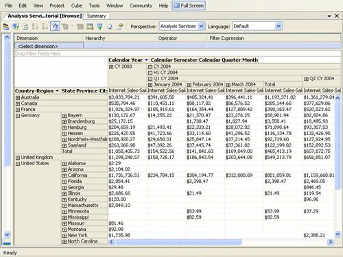
Measure can be analyzed by one or multiple dimensions. Table 15.1 earlier in this chapter is a simple example of aggregations or an OLAP report. In Table 15.1, Internet Sales-Sales Amount is a measure and Country-Region is a dimension. Thus, the data in Table 15.1 is analyzed and aggregated by a single dimension. Data can also be analyzed by two dimensions, such as date and geography, as shown in Table 15.3.
Table 15.3. Two-Dimensional Data
| Internet Sales-Sales Amount | Calendar Year | ||||
|---|---|---|---|---|---|
| Country-Region | 2001 | 2002 | 2003 | 2004 | Grand Total |
| Australia | 1,309,047 | 2,154,285 | 3,033,784 | 2,563,884 | 9,061,000 |
| Canada | 146,830 | 621,602 | 535,784 | 673,628 | 1,977,844 |
| France | 180,572 | 514,942 | 1,026,325 | 922,179 | 2,644,018 |
| Germany | 237,785 | 521,231 | 1,058,406 | 1,076,891 | 2,894,312 |
| United Kingdom | 280,335 | 583,826 | 1,278,097 | 1,195,895 | 3,338,153 |
| United States | 1,111,805 | 21,34,457 | 2,858,664 | 3,338,422 | 9,443,348 |
| Grand Total | 3,266,374 | 6,530,344 | 9,791,060 | 9,770,900 | 29,358,678 |
It is possible to add a third dimension (and so on) and, as in geometry, the structure will be a cube. A cube is basically a structure in which all the aggregations of measures by dimensions are stored.
Some dimensions can have one or many hierarchies for its members . For example:
-
Geography dimension might have a hierarchy: country, region (such as east, central, mountain, west), state (such as Texas, Florida, California), county, city, and postal code.
-
Time might have a hierarchy: year, half-year (or semester), quarter, and month.
An example of a hierarchy is demonstrated in Figure 15.1.
Figure 15.1. Multidimensional data with hierarchies.
The following walk-through should help you achieve a better understanding of OLAP and its subsequent use by Reporting Services.
| 1. | Start Business Intelligence Development Studio and create a new Analysis Services project. Give it a name Analysis Services Sample. |
| 2. | In Solution Explorer, right-click Data Sources, and select New Data Source from the shortcut menu. The Data Source Wizard begins. You can think of Data Source as a connection to the database. Click Next on the Welcome screen. |
| 3. | On the Select How to Define the Connection screen, click the New button. Enter the requested information. To connect to SQL Server database, select Native OLE DB\SQL Native Client as the Provider. |
| 4. | Enter the server name (for the local server, you can use either server name, localhost or "." dot). Select the authentication (Windows authentication is preferred). Select or enter AdventureWorksDW as the database. |
| 5. | Click Next. On the Impersonation Information screen, enter impersonation information. Selecting Use the Service Account should work in most of the cases. Leave the default name for the data source: Data Source Adventure Works DW. |
Now that you have created a data source, the next set of steps is to create a Data Source view:
| 1. | In Solution Explorer, right-click Data Source Views and then select New Data Source View from the shortcut menu. Click Next and select Adventure Works DW as the data source. Click Next. |
| 2. | The wizard examines the data source and brings up a dialog box in which tables or views from the data source can be selected. Select FactInternetSales , DimCustomer , DimGeography , and DimTime . Click Next. In the Completing the Wizard screen, enter Adventure Works DW Source View. Click Finish to complete the wizard. |
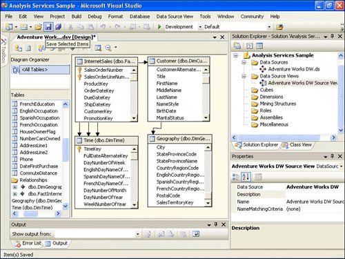
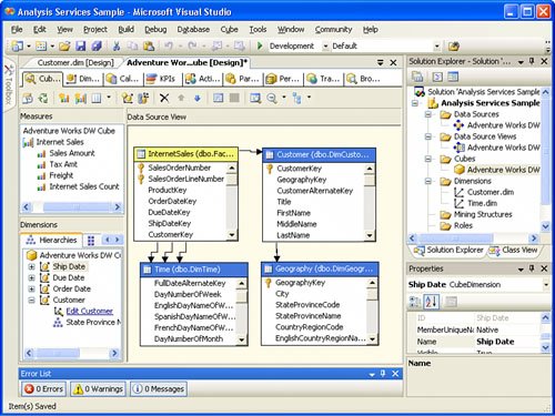
| 3. | BI/Visual Studio brings up the design diagram. The next step is to create friendly names . Right-click FactInternetSales, and then select Properties from the shortcut menu. Remove the prefix "Fact" in the Friendly Name property. For all other tables in the diagram, remove the prefix "Dim" in the Friendly Name property. After completion of this step, BI Studio looks similar to Figure 15.2. Figure 15.2 basically shows an essence of the Unified Data Model. You can connect to various data sources, create calculated fields, and establish relationshipsall without any changes to the original data. Unlike in previous versions, flattening and denormalizing of analysis data are no longer required. |
Figure 15.2. Unified Data Model.
In the next set of steps, you will create a new Analysis Services cube:
| 1. | In Solution Explorer, right-click Cubes, and then select New Cube from the shortcut menu. After reading the information, click Next on the Welcome screen. Accept the defaults on the Select Build Method screen: Build the Cube Using Data Source, Auto Build, and Create Attributes and Hierarchies. On the Select Data Source View screen, accept the default: Adventure Works DW Source View. Click Next. After processing completes, click Next on the Detecting Fact and Dimension Tables screen. |
| 2. | On the Identify Fact and Dimension Tables screen, select Time as the Time dimension table. It should look similar to Figure 15.3. The Cube Wizard looks at the data model that you have designed in Data Source view and determines the correct fact and dimension tables. Figure 15.3. Fact and dimension tables. |
| 3. | In the Select Time Periods dialog box, map the time table columns as follows :
|
| 4. | Click Next and on the Select Measures screen, deselect everything, except Sales Amount, Tax Amt, Freight, and Internet Sales Count. Note that the wizard automatically selects Internet Sales when one of the measures (for example, Freight) is selected. Only numeric values are shown for the selection on this dialog box. The Internet Sales table contains other nonnumeric columns, such as Order Number. Because it is nonnumeric, it cannot be selected as a measure. Note that the Customer Key is not included on this selection. This is because the wizard knows that it is a relationship, based on the Data Source view and does not include it in aggregations. Also note several columns with the word "Key" in their names. These are relationship columns. The wizard displays these as measures because the columns are numeric and you did not include tables that those columns reference in the Data Source view. Hence, the wizard made an assumption that the column must be a measure. Lastly, note that Internet Sales Count is not a column in the Internet Sales table, it is automatically generated by Analysis Services. Internet Sales Count represents the number of line items sold on any given level. |
| 5. | Click Next. The wizard detects hierarchies. Click Next. Note that there are only two dimensions in the Review New Dimensions window: Customer and Time. If you expand Customer, you would notice that Geography is a hierarchy under the Customer dimension. Geography is not an independent dimension because there is no direct relationship between Internet Sales and Geography, only through Customer. See Figure 15.4. You can also expand the Attributes folders to see Customer's attributes, such as First Name and Last Name. Figure 15.4. Reviewing new dimensions. |
| 6. | Click Next and name the cube Adventure Works DW Cube. Click Finish to complete the wizard. You should see a screen similar to Figure 15.5. |
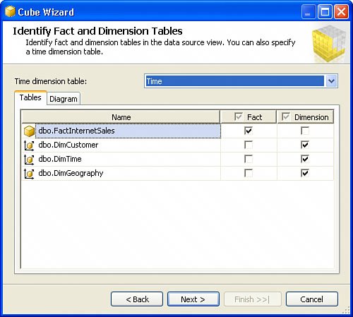
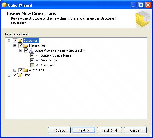
Figure 15.5. Cube design screen.
Now let's modify the Customer dimension to create a more logical Geography hierarchy than the wizard detected for us:
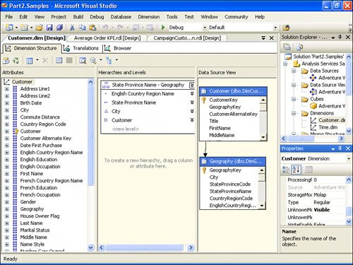
| 1. | Under the Dimension folder in Solution Explorer, double-click the Customer dimension. From the Attributes panel, drag the English Country Region Name attribute to the position right above the State Province Name level in the Geography Hierarchy. From the Attributes panel, drag the City attribute to the position right below the State Province Name level. When thinking about a hierarchy and what level to place a particular attribute, consider what "contains" or "has" what. For example, country has many states and, thus, should be on the higher level compared to state. Correspondingly, on the diagram, Country should receive less schematic "dots" than state. |
| 2. | Right-click the Geography level from the State Province Name-Geography hierarchy and select Delete from the context menu. Geography level is a geography key that does not carry useful information for our business analysis. Customer has many attributes, which might not be useful for the high-level analysis that we are trying to do. You should see a screen similar to Figure 15.6 after this step is completed. |
Figure 15.6. Dimension design screen.
The following steps will modify the Time dimension to properly order months of the year. Alphabetically, months are ordered such as: April, August, and so on. After ordering by key in place, you obtain correct ordering: January, February, and so on. You need this ordering when working with Key Performance Indicators later in this chapter.
| 1. | Double-click the Time dimension in Solution Explorer. In the Hierarchies and Levels, modify the name of the hierarchy from CalendarYearCalendarSemesterCalendarQuarterEnglishMonthNameFullDateAlternateKey to Date by right-clicking the hierarchy and selecting Rename from the shortcut menu. This is done to simplify queries that you will write in the future. |
| 2. | In the Attributes pane, click on the EnglishMonthName attribute of a Time dimension. In the Properties window (normally docked in the lower-right corner), click the KeyColumns property and click the ellipses (...). This brings up the DataItem Collection Editor dialog box. |
| 3. | Click the Remove button to delete the existing member DimTime.EnglishMonthName. Click the Add button to add a new member. In the DataItem Collection Editor under the Misc pane, click Source and then click the ellipses (...) next to Source. The Object Binding dialog box opens. |
| 4. | In the Object Binding dialog box, select ColumnBinding as the Binding type and MonthNumberOfYear as the Source column. Click OK to complete the Object Binding dialog box. |
| 5. | Make sure that the OrderBy property has the value Key. |
Now you are ready to deploy your solution:
| 1. | On the main menu, select Build, Deploy Solution. After deployment completes, double-click the Adventure Works DW Cube in Solution Explorer, and then click the Browser tab, which is the last tab in the Adventure Works Cube [Design] window. |
| 2. | Use the Reconnect button to refresh the Browser tab. Keep in mind that after the cube structure is modified and changes are deployed, you should use the Reconnect button to browse the most recent updates. BI Studio should show something similar to Figure 15.7. |
Figure 15.7. Cube browser.
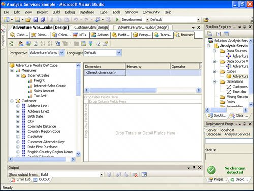
To see the results of your work, drag and drop the Sales Amount from the Internet Sales measure to the center of the pivot table control, where it says "Drop Totals or Details Fields Here." Drag and drop English Country Region Name from the Customer dimension on the row part of the pivot table control, where it says "Drop Row Fields Here." The pivot table should display information similar to Table 15.1. You have now completed and verified the cube. This is a very basic cube that will help you to understand how to use Reporting Services with Analysis Services. More details about cubes and advanced features of Analysis Services can be found in the SQL Server Books Online.
One of the new features added in Analysis Services 2005 that has high potential for use in Reporting Services is Key Performance Indicators (KPIs). Key Performance Indicators are designed to evaluate performance criteria that a business, usually, considers strategic in nature. Performance is evaluated against a specified goal and has to be quantifiable. Some of the KPI examples are: stock performance, cost of operations, customer satisfaction, and so on.
Let's add a KPI to the just-completed cube:
| 1. | In Solution Explorer, double-click the Adventure Works DW Cube. Click the KPIs tab. Right-click the surface of the KPI Organizer pane, and select New KPI from the shortcut menu. Name this KPI Average Item Price. This KPI is useful, for example, if Adventure Works' management had determined that Internet sales have the minimum order-processing costs when an average price per item sold is $100 or more. In turn , maximum order-processing cost is when the average price per item sold is less than $10. |
| 2. | For the Value Expression, enter the following MDX query: [Measures].[Sales Amount]/[Measures].[Internet Sales Count] |
| 3. | For the Goal Expression, enter 100. |
| 4. | For the Status Expression, enter the following query: Case When [Measures].[Sales Amount]/[Measures].[Internet Sales Count] < 10 Then -1 When [Measures].[Sales Amount]/[Measures].[Internet Sales Count] <= 50 Then 0 When [Measures].[Sales Amount]/[Measures].[Internet Sales Count] >= 100 Then 1 End |
| 5. | In the Trend Expression, enter the following MDX query. This query compares current values of the average order size to the previous time period (depending on the level of detail, this could be a year, month, and so on). If the current period exceeds the previous one, the trend is good; otherwise , it needs improvement. Case When ([Order Date].[Date], [Measures].[Sales Amount]) / ([Order Date].[Date], [Measures].[Internet Sales Count]) >= ([Order Date].[Date].PrevMember, [Measures].[Sales Amount]) / ([Order Date].[Date].PrevMember, [Measures].[Internet Sales Count]) Then 1 Else -1 End |
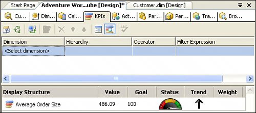
| 6. | Click the Browser View button on the KPI toolbar. Click the Process button on the KPI toolbar, and then click Run in the dialog box. Analysis Services processes KPI. After the process has completed, close the Process Progress and Process Cube dialog box. In the browser view, you should see KPI indicators, similar to Figure 15.8. |
Figure 15.8. KPIs (Key Performance Indicators).
Now let's create a mining structure. Adventure Works' management wants to create a targeting advertisement on the website to promote bicycle sales. Adventure Works had collected data from existing customers and can target those already, based on the existing data, but what about new customers making purchases? When should Adventure Works display links to bicycles to be the most effective and nonobtrusive in the advertising campaign? Similarly, what kind of customer should be targeted for a targeted mail campaign?
| 1. | In Solution Explorer, double-click Adventure Works DW Source View. Right-click in the diagram area and select Add/Remove Tables from the shortcut menu. Add the vTargetMail view. This is the view based on the data in Adventure Works DW tables, which adds a BikeBuyer field to the DimCustomer table. This field is derived from the Internet Sales table, where the product purchased was a bicycle. |
| 2. | In Solution Explorer, right-click Mining Structures, and then select New Mining Structure from the shortcut menu. Click Next on the Welcome screen. Accept the default (From Existing Relational Database or Data Warehouse) by clicking Next. Accept the default mining algorithm (Microsoft Decision Trees) on the Select the Data Mining Technique screen. Click Next. Accept the default Adventure Works DW Source View for the Data Source view. Click Next. Select vTargetMail as the Case table, and then click Next. Remember from earlier in this chapter that Case table is a table that is being analyzed to determine patterns in the data. |
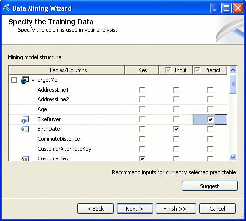
| 3. | Leave CustomerKey as the key, and then select Bike Buyer as Predictable. Note that the Suggest button has become available. Click it and note that based on the data sample, Age is the best input for the model. |
| 4. | Because the table that you have for tests does not have an Age column and to simplify further efforts, let's use Birth Date instead of Age. It is possible to use the DATEDIFF() function to calculate an age of a customer, but because Birth Date provides essentially the same (time-frame) information as Age, you can leverage Birth Date. You should see a screen similar to Figure 15.9. Click Next. Figure 15.9. Data Mining Wizard. |
| 5. | On the Specify Columns' Content and Data Type screen, click Detect. The wizard samples data. Note that the Bike Buyer's Content Type changed from Continuous to Discrete. The wizard queried the data and determined that the data is discrete, based on the fact that the Bike Buyer contains an integer value with just a few actual values: 1 and 0. Click Next. |
| 6. | In the Mining Structure name, enter Bike Buyer Structure and in the Mining Model name, enter Bike Buyer Model. Select Allow Drill Through. Click Finish. Note Customer Sales Structure appears under Mining Structures in Solution Explorer. |
Now you are ready to deploy your Data Mining Model. Click the Build, Deploy Solution menu. After deployment completes, click the Mining Model Viewer tab. Note the decision tree that was built; based on the data, it should look similar to Figure 15.10.
Figure 15.10. Decision tree.
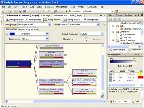
The decision tree indicates that customers born in 1969 are almost three times as likely to purchase a bike as other customers and customers born before 9/22/1931 are least likely to purchase a bike.
As an exercise to better understand data mining, click through other tabs, such as Mining Accuracy Chart. Click the Lift Chart tab under the Mining Accuracy Chart tab and note that the model provides at least 1.4 times better prediction than random guesses.
Click the Mining Model Prediction tab. Click Select Case Table on the diagram and choose vTargetMail. Drag and drop the BikeBuyer field from the Input Table on the grid located below the diagram on the screen. Drag and drop the Bike Buyer field from the mining model on the grid. On the third row of the source column, click and select Prediction Function from the drop-down menu. In the same row, select PredictProbability and drag and drop Bike Buyer from the Bike Buyer model to the Criteria/Argument column of the third row. Click the drop-down next to the Switch to Query Result View (looks like a grid) button on the toolbar and select Query. The following query is displayed. This is a DMX query comparing actual in vTargetMail table and value predicted by a model.
SELECT [Bike Buyer Model].[Bike Buyer], PredictProbability([Bike Buyer Model].[Bike Buyer]), t.[BikeBuyer] From [Bike Buyer Model] PREDICTION JOIN OPENQUERY([Adventure Works DW], 'SELECT [BikeBuyer], [BirthDate] FROM [dbo].[vTargetMail] ') AS t ON [Bike Buyer Model].[Birth Date] = t.[BirthDate] AND [Bike Buyer Model].[ Bike Buyer] = t.[Bike Buyer]
Now, you are ready to query OLAP data and data-mining structures from Reporting Services. The following are the steps:
| 1. | On the main menu, select File, Add, New Project. Select Report Server Project from the list of installed Business Intelligence Projects templates. Name the new project AnalysisServicesSamples. Click OK. Note that this is the same procedure as for creating any report project. |
| 2. | Right-click on the Reports folder under the AnalysisServicesSamples project, and select Add New Report from the shortcut menu. The Report Wizard starts. Click the Next button to advance from the Welcome screen. On the Select the Data Source screen, select New Data Source, use the name AnalysisServicesData, and select Microsoft SQL Server Analysis Services as the type of data source. Use an appropriate connection string, for example: Data Source=localhost;Initial Catalog="Analysis Services Sample" Select Make This a Shared Data Source. The Report Wizard should look similar to Figure 15.11. Figure 15.11. Analysis Services data source.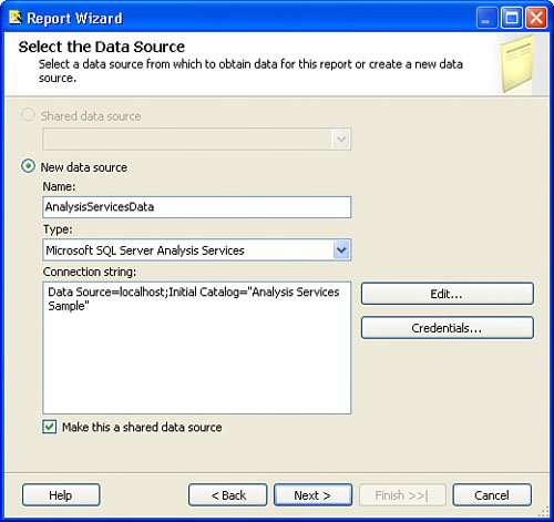 |
| 3. | Click Next. Note that the Design the Query screen does not allow you to paste in a query. This is by design to avoid potential issues with complex MDX or DMX queries. Click the Query Builder button. |
| 4. | In the Metadata pane, expand Measures/Internet Sales/Internet Sales and Customer hierarchies. Drag and drop Sales Amount from Measures on the area marked "Drag Levels or Measures Here to Add to the Query" (we will abbreviate this as "design area" from now on). Drag and drop English_Country_Region_Name on the design area. So far, the process is not very different from working with pivot tables. However, in this case, Query Builder only allows you to design queries that produce table-like output. The Query Builder should look similar to Figure 15.12. Figure 15.12. Multidimensional query designer.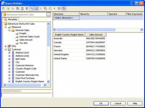 |
| 5. | Click OK and note the MDX query created by the Query Builder: [View full width]
|
| 6. | On the Select the Report Type screen, accept the default: Tabular. Click Next. On the Design the Table screen, click the Details button to add the available fields to Displayed Fields. Click Next. |
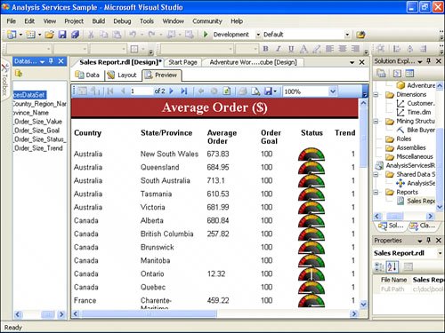
| 7. | Select Bold on the Choose the Table Style screen. Click Next. Name this report SalesReport. Click the Finish button. Click the Preview tab. You should see a screen similar to the one shown in Figure 15.13. |
Figure 15.13. Result of a multidimensional report.
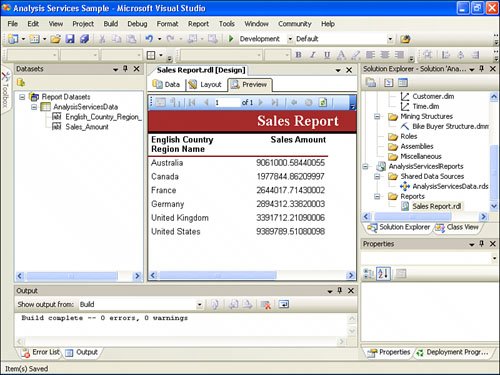
You have just pulled data from the OLAP cube.
Note
There is a bug in the RTM release of SSRS 2005 that affects OLAP reports built using the Report Wizard. If you use the Data tab, the MDX query will be lost.
The fix to this bug should be provided in the next service pack.
There are a couple of workarounds:
| 1. | You can repeat step 5 to redesign a query, using the designer provided under the Data tab. |
| 2. | Immediately after running Report Wizard, right-click on the report and select View Code from the context menu, edit the XML, and remove everything between the <rd:MdxQuery> tag and the <QueryDefinition> tag. The final code should look like this: <rd:MdxQuery><QueryDefinition ... Save the file. |
Let's make this report a bit more complicated and add a second dimension: Time. You will use the SalesReport that you have developed as a base for the following steps:
| 1. | In Solution Explorer, right-click on SalesReport and select Copy from the shortcut menu. Right-click the report project and select Paste from the shortcut menu. Rename Copy of SalesReport to TimedSalesReport. |
| 2. | Double-click TimedSalesReport and click the Data tab in Report Designer. |
| 3. | Expand the Order Date dimension. Drag and drop Calendar Year on the design area. Once again, Query Builder flattens the OLAP output. Toggle the design mode and note that the MDX query now has a second dimension. SELECT NON EMPTY {[Measures].[Sales Amount] } ON COLUMNS, NON EMPTY {([Customer].[English Country Region Name].[English Country Region Name].ALLMEMBERS * [Order Date].[CalendarYear].[CalendarYear].ALLMEMBERS ) } DIMENSION PROPERTIES MEMBER_CAPTION, MEMBER_UNIQUE_NAME ON ROWS FROM [Adventure Works DW Cube] CELL PROPERTIES VALUE, BACK_COLOR, FORE_COLOR, FORMATTED_VALUE, FORMAT_STRING, FONT_NAME, FONT_SIZE, FONT_FLAGS |
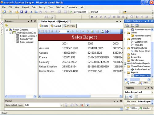
| 4. | Click the Layout tab and delete the table control from SalesReport. Place a matrix control in place of the table control. From the Datasets window, drag and drop Sales_Amount on the data region of the matrix control, drag and drop CalendarYear on the column area, and drag and drop English_Country_Region_Name on the Rows area of the matrix control. Now, you should see a screen similar to Figure 15.14. |
Figure 15.14. Result of a multidimensional report with Time dimensions.
Now let's create a report that leverages Key Performance Indicators (KPIs). Once again, you will use the SalesReport that you have developed as a base for the following steps:
| 1. | In Solution Explorer, right-click on SalesReport and select Copy from the shortcut menu. Right-click the report project and select Paste from the shortcut menu. Rename Copy of SalesReport to ItemPriceKPI. |
| 2. | Double-click ItemPriceKPI and click on the Data tab in Report Designer. Right-click in the design area and select Clear Grid from the shortcut menu. In the metadata, expand KPIs. Drag and drop the Average Item Price KPI on the design area. The design area now shows a grid with a single row with four columns corresponding to the details of KPI: Average Item Price Value, Average Item Price Goal, Average Item Price Status, and Average Item Price Trend. |
| 3. | From the Customer dimension, drag and drop State_Province_Name. Click on Layout view and if it has a table or matrix control, delete it. Add a new table control. Add two more column to the table. Drag and drop English_Country_Region_Name, State_Province_Name, Average_Item Price_Value, Average_Item_Price_Goal, and Average_Item_Price_Status fields from the AnalysisServiceData data set to the Detail region of the table. Click the Preview tab. You should see a screen similar to Figure 15.15. |
Figure 15.15. Result of a multidimensional report with KPIs.
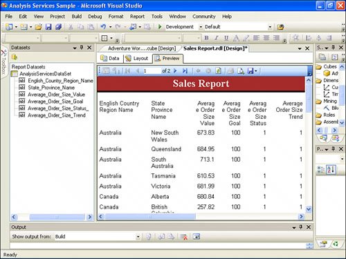
You can validate the status works well and displays 1 when Average Order Size > 100, 0, and when it is <= 50, and display -1 when the Average Order Size is < 10.
Note that all the KPI data is numeric. This version of Reporting Services does not include KPI controls, but KPI controls are easy to emulate. The following several steps show how to do it. You can create your own KPI graphics or leverage KPI controls from Visual Studio (by default located at C:\Program Files\Microsoft Visual Studio 8\Common7\IDE\PrivateAssemblies\DataWarehouseDesigner\KPIsBrowserPage\Images ).
Let's embed three images Gauge_Asc0.gif , Gauge_Asc2.gif , and Gauge_Asc4.gif corresponding to three distinct states of the gage's status: empty, half, and full. The steps to emulate KPI controls are as follows:
| 1. | From the Toolbox, drag and drop an image control on the Detail area of the grid inside of the column Status. The Image Wizard begins. On the Welcome screen click Next, select Embedded Image on the Select the Image Source screen, and then click Next. If there are no embedded images, click Add New Image and add images. After you are done, click Finish. |
| 2. | Click the image and in the Properties window, change the Value property from gauge_asc4 to the following expression: =IIF (Fields!Average_Order_Size_Status_.Value=-1, "gauge_asc0", IIF(Fields!Average_Order_Size_Status_.Value=0,"gauge_asc2","gauge_asc4") ) As you can tell by now, this expression directs Reporting Services to display an appropriate image. Note that image names are displayed as constants in the Expression Editor. Do not forget to include image names in double quotes, such as "gauge_asc0" . You should see a screen similar to Figure 15.16. Figure 15.16. Adding graphical KPIs.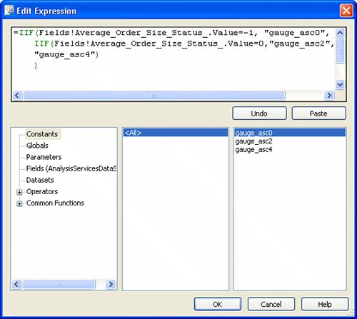 |
| 3. | Click OK to close the Expression Editor. |
| 4. | If desired, you can modify formatting, such as the column headers to improve the report's look. Click the Preview tab. You should see a screen similar to Figure 15.17. This approach to adding images would just as easily work with reports from relational data. |
Figure 15.17. Resulting report after adding graphical KPIs.
You might have noticed that in the KPI example Brunswick in Canada, for example, does not have sales data (that is, nothing was sold there). In the real-life report, you should have excluded output of empty (or irrelevant data). Such filtering should be done, ideally , in a query. Report Server could be leveraged as well, for example, using the Visibility property of a report item.
Creating Data-Mining Reports
As a last exercise in this chapter, let's create a report that will leverage Data Mining capabilities of SQL Server:
| 1. | In Solution Explorer, right-click the Reports folder and select Create New Report from the shortcut menu. Use the AnalysisServicesData shared data source that was created earlier in this chapter. Click Next. |
| 2. | On the Design the Query window, click the Query Builder button. By default, Query Builder starts in MDX Query Design mode. To switch to DMX Query Design mode, click the third button on the Query Builder's toolbar, which is called Command Type DMX (this button depicts a mining pickax). This button switches between MDX and DMX designer to correspondingly query OLAP cubes and data mining models. Click OK on the warning dialog box. |
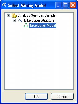
| 3. | On the Mining Model window, click the Select Model button. Expand the tree and select the Bike Buyer Model. On the Select Input Table(s) window, click Select Case Table (see Figure 15.18). Figure 15.18. Select Mining Model window. |
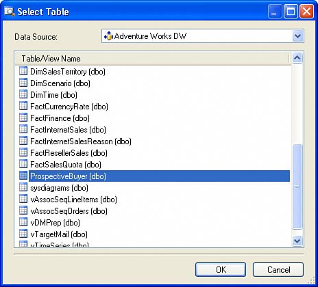
| 4. | Change the data source to Adventure Works DW, select ProspectiveBuyer (see Figure 15.19), and then click OK. Figure 15.19. Selecting a table for analysis. |
| 5. | Drag and drop Bike Buyer from the Bike Buyer model to the grid below; in the source column of the second row of the grid, select Prediction Function in the drop-down menu within a cell. In the Field column, select the PredictProbability function; and drag and drop the Bike Buyer field from the model to the Criteria/Argument field column. Enter Probability as an alias for this expression. |
| 6. | From the ProspectiveBuyer table (located in Select Input Table window), drag the following fields: FirstName, LastName, and EmailAddress. This allows you to have a report that can be used for a personalized email campaign promoting Adventure Works' bikes. You should see a screen similar to Figure 15.20. Figure 15.20. DMX Query Builder.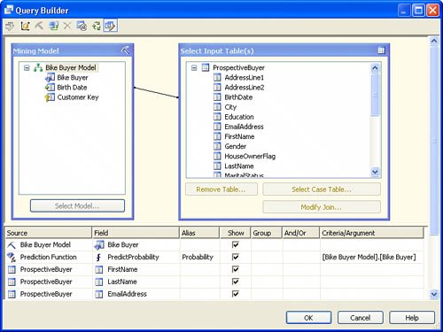 |
| 7. | Click OK to complete Query Builder. The following is the query: SELECT [Bike Buyer Model].[Bike Buyer], (PredictProbability([Bike Buyer Model].[Bike Buyer])) as [Probability], t.[FirstName], t.[LastName], t.[EmailAddress] From [Bike Buyer Model] PREDICTION JOIN OPENQUERY([Adventure Works DW], 'SELECT [FirstName], [LastName], [EmailAddress], [BirthDate] FROM [dbo].[ProspectiveBuyer] ') AS t ON [Bike Buyer Model].[Birth Date] = t.[BirthDate] |
| 8. | On the Select Report Type screen, accept the default Tabular by clicking Next, and add all the fields to Details in the Displayed Fields section. Click Next, and accept the default style by clicking Next. Name the report CampaignCustomerEvaluation. Format the fields to improve layout and click Preview. The screen should look similar to Figure 15.21. Figure 15.21. Data-mining report.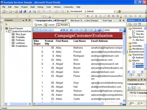 |
EAN: 2147483647
Pages: 254