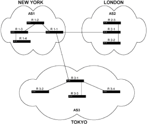
Chapter 4 - Routing Protocols Used in TCPIP

Chapter 4: Routing Protocols Used in TCP/IP

	Objectives

	This chapter examines various routing protocols popular in the TCP/IP world. By the end of this chapter you should have a good theoretical understanding of the following protocols and know how they are implemented in a Cisco environment.

			RIP version 1

			IGRP

			EIGRP

			OSPF

			Integrated IS-IS

			EGP and BGP

Additionally, you should be able to choose which routing protocol to use for different situations. Finally, the process of redistribution, which enables multiple routing protocols to communicate on one internetwork, will be explained, and examples of implementation given. We will discuss the theory of each protocol, its good and bad points, and examine how the protocol can be configured on Cisco routers.

Routing Protocol Responsibilities

	Routing protocols exist to keep routing tables accurate, even though the internetwork they are operating on will be changing due to equipment or line failures and the addition of new network segments.

	To keep tables accurate, a routing protocol operation has two parts. The first sends advertisements (referred to as routing updates) out from a router, regarding the location of network numbers it knows about. The second receives and processes these routing updates in a way that keeps the router's routing table directing traffic efficiently.

	There are two main types of routing protocols, the Interior Gateway Routing Protocol and the Exterior Gateway Routing Protocol. To understand the difference between these two, we need to define what an autonomous system is on an internetwork. Figure 4-1 shows a large internetwork split into three autonomous systems.

	Figure 4-1: An internetwork split into three autonomous systems

	The idea behind autonomous systems is as follows. Imagine there are three different internetworks, one managed by an American-based team, one by a UK-based team, and one by a team based in Japan. Each of these internetworks is managed in a different way and has different policies. Suppose these three internetworks need to be connected so they can exchange information, but the separate network management teams want to retain their own policies and want to control the routing updates received from the newly connected internetworks.

	One way to meet these goals is to define an Exterior Gateway Routing Protocol process on the routers that connect the three internetworks. In Fig. 4-1, these are routers R1-1, R2-1 and R3-1. The Exterior Gateway Protocol limits the amount of routing information that is exchanged among these three internetworks and allows them to be managed differently.

	Within each autonomous system, all routers would run an Interior Gateway Routing Protocol, which assumes that the whole internetwork is under the management of one body and, by default, exchanges routing information freely with all other routers in the same autonomous system. Sophisticated Interior Gateway Routing Protocols, such as Cisco's IGRP, however, have the functionality to act as Exterior Gateway Routing Protocols. As with most things in computer networking, clear-cut definitions are hard to come by.

	Exterior Gateway Routing Protocols and multiple autonomous system numbers are used on the Internet but rarely in the commercial environment, so we shall concentrate mainly on the Interior Gateway Routing Protocols in this chapter.

	The world of Interior Gateway Routing Protocols is split into two camps, one known as distance vector and the other as link state. In the next section, we discuss two distance vector routing protocol algorithms, RIP and IGRP, followed by a discussion of the hybrid EIGRP. After that, we shall look at two link state protocols, OSPF and Integrated IS-IS.

Interior Gateway Protocols: Distance Vector

	The first distance vector protocol was the Routing Information Protocol, (RIP). The discussion that follows on RIP fully explains how a distance vector routing protocol works. We will review the generic distance vector algorithm, followed by discussion of RIP version 1 as the first protocol of this type.

	Generic Distance Vector

	The distance vector algorithm (sometimes referred to as the Bellman-Ford algorithm for the people who invented it), requires each machine involved in the routing process to keep track of its "distance" from all other possible destinations. What happens is that a router is programmed to construct a table of all possible destinations (in terms of network numbers) and measure the distance to each location. The only information a router has at boot time is what networks are directly attached to it. So how can it find out about all other possible destinations?

	Each router is programmed so that it announces all the destinations it knows about, along with the distance to each. Once a router starts hearing all the advertisements from other routers, it can start to list all the possible destinations and calculate the shortest path to these destinations the one kept in the routing table.

	So a distance vector protocol will, on a regular basis, send out an update that contains all the information contained in the machine's routing table. These updates are sent only to neighboring routers on directly connected segments. One of the key differences between distance vector and link state routing is that link state protocols send information to routers on remote segments.

	Once these updates get to a router, the router will then use a collection of algorithms and timers to decide what entries should be put into the routing table of the machine that is receiving the updates. Another key aspect of distance vector protocols is that any given machine knows only the next hop in the sequence to deliver the packet to its ultimate destination. In link state protocols, each machine has a complete map of the network it is in (or, more accurately, the routing area it is in but we will come to that later).

	To finish this introduction, let's take a high-level overview of the code behind the distance vector algorithm:

	1.		Each router has a unique identification on the internetwork.

	2.		Every router will identify a metric to be associated with each link directly connected to itself.

	3.		All routers will start advertising directly connected links with a metric of zero.

	4.		Every router transmits to neighbors the complete information regarding all destinations and their metric when the router first boots, then periodically, and whenever a router becomes aware of a change.

	5.		Each router determines which directly connected neighbor offers the lowest metric to each location.

	RIP: The Routing Information Protocol

	The first Interior Gateway Protocol (IGP) was the Routing Information Protocol, or "RIP" as it became known. RIP was designed for an environment that had only a relatively small number of machines, and these machines were connected with links that had identical characteristics.

	As the first IGP, RIP gained widespread use and was distributed free with BSD Unix as the routed daemon process. As today's heterogeneous networks grow and become more diverse, RIP has been improved upon with more modern, more full-featured distance vector protocols. RIP is still in widespread use and is the only routing protocol that Unix machines universally understand.Okay, before we get into the workings of RIP, let's refresh our memories regarding what a routing table looks like. To display a Cisco router's routing table, do the following:

	C - connected, S - static, I - IGRP, R - RIP, M - mobile, B - BGP

D - EIGRP, EX - EIGRP external, O - OSPF, IA - OSPF inter area

E1 - OSPF external type 1, E2 - OSPF external type 2, E - EGP

i - IS-IS, L1 - IS-IS level-1, L2 - IS-IS level-2, * - candidate default

Gateway of last resort is not set

	160.4.0.0 255.255.255.224 is subnetted, 2 subnets

C  160.4.1.32 is directly connected, Ethernet0

R  160.4.1.64 [120/1] via 160.4.1.34, 00:00:12, Ethernet0

	In the first column, the router tells us how it learned about the routing table entries. The legend at the top of the display explains what these abbreviations mean. For example, C means that the network is directly connected to the router on the specified interface. S stands for static route and means that the route to this destination network is hard-coded into the router's configuration. R means that the router learned of this destination network via a RIP update.

	The rest of the entry in the router's routing table states which interface to use for the specified network, and which router to send the packet to next if the destination network is on another part of the internetwork. In this case, the RIP entry is telling us to use the router with address 160.4.1.34 in order to get to the 160.4.1.64.subnet, and that this router is connected to the Ethernet 0 interface.

	Let's look at the rest of this entry in more detail. The [120/1] entry in the RIP line first gives the value of the administrative distance, and then the metric. The administrative distance is a value assigned to routing protocols. RIP has a value of 120, OSPF of 110, IGRP of 100, EIGRP of 90, static of 1, and directly connected of 0.

	This administrative distance is used if two routing protocols advertise the same route to the same router. In this case, the router will prefer the route supplied by the routing protocol with the lowest value for administrative distance. The logic behind this is that, because Cisco routers give you the ability to have multiple routing protocols running on the same router, you need some way of deciding which routing protocol is advertising the best route. Clearly the metrics used by different routing protocols are not comparable; RIP only goes up to a metric of 16, while IGRP goes to more than 16 million, so this other measure is used to show preference for the routing protocols in use. EIGRP is most preferred, IGRP next, then OSPF and finally RIP.

	The 00:00:12 value is a counter that indicates the amount of time that has passed since the router received an advertisement for this route.

	We will now discuss how RIP handles its responsibilities as a routing protocol in more detail.

	The Basics of How RIP Works.     Once configured on an internetwork, the operation of RIP and its interaction with the routing table is fairly straightforward. By default, every 30 seconds each RIP-enabled device sends out a RIP update message, comprising routing information from the machine's routing table. This message includes the following:

			Destination address of host or network.

			The IP address of the gateway sending the update.

			A metric that indicates the distance (in terms of hops) to the destination.

	It is worth noting that interfaces on a Unix machine or a router can be defined as passive. If that is done, the interface in question does not send out any RIP updates; it merely listens for updates from other machines.

	Once a routing device receives an update, it processes the new information, which it compares with that in the existing routing table. If the routing update includes a new destination network, it is added to the routing table. If the router receives a route with a smaller metric to an existing destination, it replaces the existing route. If an entry in the update message has the same destination network and gateway but a different metric, it will use the new metric to update the routing table.

	This covers how routers handle a static network using RIP; some additions to the protocol are in place to handle changes in topology, such as a downed link. If the preceding were the only logic coded into a router, it would not recover from a downed link because it remembers only the best route to any given destination. If the gateway, or link to that gateway, should fail, the routing table might never reflect the change.

	That's because, so far, the logic defined depended upon a gateway notifying its neighbors of whether its metrics had changed. If the gateway could no longer communicate, it could not notify its neighbors of a change. To handle such situations, RIP employs timers: It sends out messages (every 30 seconds by default), and the protocol assumes that if a gateway or specific route is not heard from within 180 seconds, it no longer is available. Once it determines that a route is unavailable, the router sends a special message that notifies its neighbors of the unavailable route. After 270 seconds, if nothing is heard from the gateways or route, this information is flushed from the router's routing table. These timers are known as the update, invalid, and flush timers, respectively.

	To understand fully how a router deals with link or other failures on the internetwork, we need to explore other issues, starting with the count to infinity problem. With a router that uses RIP as its routing protocol, "infinity" turns out to be 16. Clearly, some further explanation is needed here.

	RIP's interpretation of infinity as the number 16 relates to the Time To Live (TTL) field in the IP layer header. Each time a packet travels through a router, its TTL field (with initial value of 15) is decreased by one. When the TTL value reaches 0, the packet is discarded and no longer exists in the internetwork. This feature is there to stop a packet caught in a routing loop from being switched back and forth forever between routers. Obviously we want the TTL value to be high enough to allow us to send correctly routed packets through whatever network size we want to implement, but small enough so that packets are not kept in a routing loop for too long. In a RIP-based network, this value is fixed at 15. With IGRP, we can set the value to whatever we like.

	Let's see how this situation of a circulating packet can occur, and what features in RIP have been implemented to minimize its occurrence. Referring to Fig. 4-2, consider the situation wherein a PC on network 3 needs to send a message to a PC on network 1.

	Figure 4-2: An internetwork in which Split Horizon prevents routing loops

	First let's examine what happens with RIP during normal operation. Router A initially will advertise that it knows about networks 1 and 2. Router B will advertise that it knows about networks 2 and 3. (This is similar to the lab we set up in Chap. 3.) After these initial advertisements, both routers know about all three networks. If router B sends an update to router A, stating that it knows how to get to network 1, we can run into some problems. Here's how this can happen.

	Suppose the interface on router A goes down and router A cannot contact network 1. If router B is advertising to router A a route to network 1, router A will think that it can get to network 1 by sending a packet to router B. So, if a PC on network 3 wants to send a packet to a PC on network 1 and the interface on router A to network 1 goes down, the packet will get caught in a routing loop. This happens because router B will decide that to get to network 1, it must send the packet to router A. Router A knows that its directly connected interface to network 1 is down and that network 1 cannot be reached that way. Since router A has received an update from router B stating that it knows how to get to network 1, the packet will get sent back to router B and the process starts all over. The only thing that stops this process is the count to infinity.

	The Split Horizon algorithm was designed to counter this problem. The effect of the Split Horizon rule is that a router will send out different routing update messages on different interfaces. In effect, a router never sends out information on an interface that it learned from that interface. The logic is that if a router first learns of a network from an adjacent router, that adjacent router must be nearer the network. The effect of this rule in the sample internetwork of Fig. 4-2 is that router B will have learned about network 1 from router A, and therefore, according to Split Horizon, router B will not include network 1 in its routing updates sent to router A.

	RIP version 1 implemented Split Horizon with Poison Reverse Update. This formidable-sounding title is, in fact, a small modification to the Split Horizon algorithm described above. All it means is that, instead of not advertising routes to the source, routes are advertised back to the source with a metric of 16, which will make the source router ignore the route. It is perceived that explicitly telling a router to ignore a route is better than not telling it about the route in the first place.

	All this means in practice (if the fault condition is in effect) is that a PC will know that it cannot send a message to a PC on network 1 more quickly. This could mean that a user knows he cannot send his message, or this knowledge could kick off some dial-backup facilities to restore service more quickly.

	Split Horizon, with or without Poison Reverse, only counters routing loops between adjacent routers. Let's look at Fig. 4-3 and see a situation in which Split Horizon will not save us from a routing loop.

	Figure 4-3: An internetwork in which RIP's maximum metric value causes problems

	Suppose router C gets a packet destined for network 1; then, in normal operation, the packet is sent to router A for delivery. If the interface on router A to network 1 goes down, router A knows it cannot deliver the packet to network 1 directly and will seek an alternate route. Split Horizon stops router C from telling router A that it knows how to get to network 1, but it will tell router B. After the network 1 interface failure on router A, router B will no longer hear about network 1 from router A, but will hear about it from router C. Therefore, router B will be free to advertise a route to network 1 to router A, stating that it can get to network 1 via router C. This leads to a routing loop between routers A, B, and C, even though Split Horizon is in effect.

	Another time when the value 16 has significance in a RIP-based network is when a network has been built that has a path through more than 15 routers from source to destination.

	Router D will hear about two ways to get to Network 1, one from router A and one from router C. Router A will advertise network 1 to both C and D with a metric of 1. Router C will increment this metric by 1 (to indicate the packet has traveled through a router) and will readvertise this route to D. Router D will get both of these updates and select router A as the best way to get to network 1, because it has the lowest metric. Now suppose router A had received a routing update from network X, which had a route with a metric of 15. Router A will add 1 to the metric, making it 16. The next router to receive this in an update from A will declare that it is infinity and will eliminate this route from its routing table (if the route existed there in the first place) or, at the very least, fail to add this route to its routing table.

	This means that routers B, C, and D will not be able to reach anything on network X, because RIP will think that network X is too far away. This is annoying, particularly if all of the links and routers are functioning correctly.

	Triggered Updates and Hold-Downs.     The larger a network grows, the more difficult it is to get all the routing tables on all the routers updated correctly. The time it takes for all the routing tables to get adjusted by a routing protocol is called the convergence time. To speed up this process, RIP employs triggered updates, which means that whenever a RIP-enabled router learns of a topology change, such as a link becoming unavailable, it will not wait for the next scheduled routing update to be sent out, but will instead send out a triggered update immediately.

	Unfortunately, this does not work for all situations. Look at Fig. 4-4 to examine what happens if the link between A and B becomes unavailable. When routers A and B realize that they are no longer connected, they will notify their neighbors of the link failure via a triggered update. All router devices receiving this news will issue triggered updates to their neighbors, indicating the change in topology. Problems occur if, for example, router E is made aware of the change before router D. Router E adjusts its routing table to reflect that the A-to-B link is no longer available; however, if router D has not heard of this change and sends to E a regular update message (assuming that the A-to-B link is still available), E will reinstate the A-to-B link in its routing table.

	Figure 4-4: A larger internetwork in which the use of hold-downs is necessary

	In this situation, the benefit of using triggered updates has been negated, and we still have to wait for the A-to-B route to expire in all the routing tables in the network. A method for improving the convergence time in this type of situation is the hold-down timer.

	The hold-down rule states that when a route is removed, no update to that route will be accepted for a given period of time. In our example, this means router E will ignore the update from router D attempting to reinstate the A-to-B route. This gives the triggered updates time to get to all other routers, ensuring that any new routes are not just reinstating an old link. The downside of this scheme is that the system will not reach convergence in the quickest possible time. However, convergence time with triggered updates and hold-downs is much better than without.

	Now that we have explained the operation of RIP, we can go back to the lab and explore the information that the router will give us regarding RIP.

	The command show ip route 160.4.1.64 gives some expla-nation of the summarized display given when a Show ip route is executed.

	router1#sho ip route 160.4.1.64

Routing entry for 160.4.1.64 255.255.255.224

Known via "rip", distance 120, metric 1

Redistributing via rip

Last update from 160.4.1.34 on Ethernet0, 00:00:26 ago

Routing Descriptor Blocks:

* 160.4.1.34, from 160.4.1.34, 00:00:26 ago, via Ethernet0

Route metric is 1, traffic share count is 1

	The point of interest is that the display tells us the netmask used in determining subnet values, in this case 255.255.255.224. In addition, it explains that the 120 value is the administrative distance and the metric is 1. Further, it explains that the last update for this route was obtained 26 seconds ago from address 160.4.1.34 on Ethernet 0.

	The next command, show ip protocols, gives us the timer values, discussed in the preceding section, for this specific RIP system.

	router1#sho ip protocols

Routing Protocol is "rip"

Sending updates every 30 seconds, next due in 22 seconds

Invalid after 180 seconds, hold down 180, flushed after 240

Outgoing update filter list for all interfaces is not set

Incoming update filter list for all interfaces is not set

Redistributing: rip

Routing for Networks:

160.4.0.0

Routing Information Sources:

GatewayDistanceLast Update

160.4.1.341200:00:16

Distance: (default is 120)

	Problems with RIP.     In today's large, heterogeneous networks that connect Ethernet segments to serial-line wide area links and dial-up links, the following problems make the use of RIP far from ideal.

			As the network grows, destinations that require a metric of more than 15 become unreachable. This is particularly bad if a network administrator applies a metric of more than 1 to a link, to indicate a slow transmission time.

			The overly simplistic metric generates a suboptimal routing table, resulting in packets being sent over slow (or otherwise costly) links when better paths are available. Other routing protocols use a more complex metric to include the throughput of each link in use.

			RIP-enabled devices will accept RIP updates from any device. This enables a misconfigured device to disrupt an entire network quite easily. Other protocols allow "neighbors" to be defined as the only ones from which to accept routing updates.

			RIP does not carry subnet mask information in updates. It assumes all interfaces on the network have the same mask. Because of this, the network can run out of usable Internet-compatible addresses earlier than is necessary.

			On larger internetworks, convergence time is unacceptably slow (greater than 5 min) for most commercial applications such as database access or financial transactions.

			The Split Horizon with Poison Reverse Update algorithm in RIP only counters routing loops between adjacent routers. Other routing protocols employ more sophisticated mechanisms to counter larger routing loops, thereby allowing the safe use of a zero hold-down value, which speeds up convergence time considerably.

			RIP updates use more bandwidth than other protocols, mainly because the whole routing table is sent in updates.

	Even though it may not be the best protocol available, there are still those who have to introduce Cisco routers into a largely Unix-based routing environment, and the only routing protocol that routers can use to exchange information reliably with Unix machines is RIP. With that in mind, let's see what needs to be done to configure RIP on a Cisco router.

	The first step is to enable the process on the router, which is achieved as follows:

	Router1(config)#router rip

Router1(config-router)network A.B.C.D

	The first line defines RIP as a running process, and the second defines the whole network number that will be advertised by RIP on initial startup of the routing process. You need to add entries for all the network numbers that are directly connected. If there may be interfaces on the router that you do not want to send routing updates through, consider Fig. 4-5.

	Figure 4-5: The use of passive interfaces on a RIP internetwork

	In this figure, the Ethernet 0 port is connected to a local area network. This network may contain routers advertising routes that you do not want to get to the global wide area net. To stop the router sending any of these local routes over the global net, use the passive interface command as shown next. This command stops the router from sending out any updates on the specified interface.

	Router1(config-router) #passive interface SO

	RIP is a broadcast protocol, so in order for routing updates to reach routers on nonbroadcast networks, you must configure the Cisco IOS to permit this exchange of routing information. This is a fairly rare occurrence. Consider Fig. 4-6.

	Figure 4-6: Configuring RIP to send routing updates to a specified router

	Suppose you have two sites connected via a public frame relay network and want router 1 to send RIP updates to router 2. With a default configuration for RIP, the frame relay network will not broadcast the RIP update to all connected devices, so we have to tell router 1 to send a directed RIP update message to router 2. This is achieved as follows:

	where W.X.Y.Z. is the IP address of router 2.

	In summary, the RIP configuration utilizing all these features is shown as follows:

			router rip

			network A.B.C.D

			passive interface serial 0

			neighbor W.X.Y.Z

	It is possible to change the value of the update, invalid, and flush timers along with the value of hold-down. I do not recommend you do this for RIP. The only reason to use RIP on a router is if you are exchanging routing information with a Unix machine, and it is likely that the timers and hold-down value for the Unix machine are not easily configurable. If you are concerned enough about the performance of your routing protocol to adjust the timers, you should not be using RIP, but rather something such as IGRP, and use redistribution (discussed later in this chapter) to exchange route information with Unix machines.

	RIP performed its job well, given what it was designed for, but its time as the only routing protocol to run on a large and diverse network is over. Let's look at how Cisco improved things with the Interior Gateway Routing Protocol, IGRP.

	IGRP: Interior Gateway Routing Protocol

	Cisco's stated goals for IGRP include the following:

			Stable, optimal routing for large internetworks, with no routing loops occurring.

			Fast response to changes in network topology.

			Ability to handle multiple "types of service" (though not currently implemented).

			Low overhead in terms of bandwidth and router processor utilization.

			Ability to split traffic among several parallel routes when they are of roughly equal desirability.

	The key differences between RIP and IGRP are in the metric, poisoning algorithm, and use of default gateway. IGRP's Split Horizon, triggered updates, and hold-downs are implemented in a fashion similar to RIP.

	IGRP Metrics.     IGRP computes a vector of metrics that is used to characterize paths. This metric value can exceed 16 million, which allows a great deal of flexibility when mathematically describing link characteristics. This composite metric (as defined by Cisco) is calculated as follows:

	[(K1/B) + (K2xD)]xR

	where

	K1, K2 = constants

	B =

	unloaded path bandwidth x (1 channel occupancy). This is for the narrowest bandwidth segment of the path.

	D =

	Topological delay

	R =

	reliability

	Two additional data elements are passed in routing updates: hop count and Maximum Transmission Unit, although neither currently are used in the calculation.

	K1 and K2 indicate the weight to be assigned to bandwidth and delay, and are defined by the type of service requested for a packet. In reality, the metric calculation is much simpler than this equation would suggest. If two routers are connected via their Serial 0 ports, the default bandwidth assumed for the metric calculation is 1.544 Mbps (T-1 speed). For a T-1, IGRP assigns a composite delay of 21,000 ms. By default K1 = 10,000,000; K2 = 100,000; and R = 1. This gives a metric of 8576 for every serial port connection on a network, regardless of the actual line capacity in place. This metric value can be viewed by using the show ip route A.B.C.D command, in which A.B.C.D is the IP address of a device on the other side of the serial port link. An example is shown as follows:

	router1#sho ip rout 160.4.1.64

Routing entry for 160.4.1.64 255.255.255.224

Known via "igrp 9", distance 100, metric 8576

Redistributing via igrp 9

Last update from 160.4.1.34 on Ethernet0, 00:00:33 ago

Routing Descriptor Blocks:

* 160.4.1.34, from 160.4.1.34, 00:00:33 ago, via Ethernet0

Route metric is 8576, traffic share count is 1

Total delay is 21000 microseconds, minimum bandwidth is 1544 Kbit

Reliability 255/255, minimum MTU 1500 bytes

Loading 1/255, Hops 0

	Metric values can be customized using the bandwidth interface command for each serial port, to factor in actual bandwidth available for each link for metric calculations. This is a good idea.

	As stated, the Cisco IOS, unless it is configured otherwise, will decide that each serial link is using a T-1 for the purposes of metric calculation.

	This can be verified by issuing the following command on router A (see Fig. 4-7).

	Figure 4-7: Internetwork in which interface bandwidth commands are necessary

	RouterA>show interface serial 1

Serial1 is up, line protocol is up

Hardware is HD64570

Internet address is 160.4.1.65 255.255.255.224

MTU 1500 bytes, BW 1544 Kbit, DLY 20000 usec, rely 255/255, load 1/255

	The first four lines of command output are shown. As you can see, the bandwidth assumed is that of a T-1, even though a 64 kbps line is in use. It would have been nice if this bandwidth value had used what was actually there by default; because the router is getting the clock signal from the line CSU/DSU, it does have the information to do so but the connection in the Cisco IOS is not made.

	Why is this important? As previously stated, IGRP will split traffic between paths that it thinks are of equal value in terms of the composite metric. If no adjustments are manually made to the router configuration to change the value of bandwidth used for the 64 kbps links in the metric calculation, router A will calculate the metric from network 1 to network 2 as 17152 (8576 + 8576) for both the route through router D and the route through router B. Transferring a file from a machine on network 1 to a machine on network 2 will mean that the traffic is split equally between these two paths. As you can see, the available bandwidth of these two paths is actually very different, which will lead to a suboptimal rate of file transfer.

	The way to fix this is to assign appropriate bandwidth values to each link. This is achieved as follows:

	RouterA(config)#interface serial 1

RouterA(config-int)#bandwidth 64000

	The same should be done for the Serial 1 interface on router B. The result of this is that the route from network 1 to network 2 will have a far lower metric through router D than through router B. As the routes no longer have equal metrics, for a file transfer from network 1 to network 2, the path through router D will carry all the traffic.

	In the Cisco IOS, the concept of variance can be used to define unequal-cost load balancing. This means that if up to four paths are roughly equal, traffic will be split among them, in inverse proportion to their metric value. These alternative path metrics must be within a specified variance multiplier of the best metric. The variance value multiplied by the best metric defines the upper value of the metric of the links that will be considered for unequal-cost load balancing. In Fig. 4-8, we see an internetwork that, with appropriate settings of variance, will allow traffic between network 1 and network 2 to be split between routes through router B and D, in proportion to the bandwidth available.

	Figure 4-8: Internetwork in which the use of variance is recommended

	In this instance it is desirable to have traffic between network 1 and 2 split between the two paths. If the variance is set to a value greater than 1, traffic may be split over paths of unequal metric. A value of 1 is the default and means that traffic will only be sent over the best path, or split between equal paths. If the variance is set to 1.5, it means that any path with a metric up to 1.5 times the metric of the best path will be added to the routing table and used when sending traffic.

	The variance multiplier is set as follows:

	RouterA(config-router)#variance 1.5

	Caution must be taken with network design due to IGRP's ability to use load balancing. As long as either the Data Link or Transport layer protocol can handle receiving out-of-sequence packets, everything is fine. If one is using frame relay, for example, to transport UDP packets in an internetwork with multiple routes between networks, however, the IGRP feature will cause problems, because neither frame relay nor UDP guarantee correct sequencing of packets. In this instance, using TCP as the transport protocol, or swapping to LAPB for the link-level protocol, will resolve the problem.

	IGRP Route Poisoning.     The poisoning algorithm used in IGRP can counter larger routing loops than can the Split Horizon with Poison Reverse used by RIP. RIP's poisoning algorithm only counters routing loops between adjacent routers. IGRP will poison routes in which metric increases by a factor of 10 percent or more after an update. This is based on the logic that routing loops generate continually increasing metrics. Using this type of poisoning rule will mean that certain valid routes will be erroneously deleted from routing tables. If routes are valid, however, they will be reinstated by the next regular update message. The key advantage to this type of poisoning is that it safely allows a zero hold-down value, which speeds up network convergence time considerably.

	IGRP Default Gateway.     For routers, the network number 0.0.0.0 has special significance to identify a specified router as the default gateway. A default gateway is used by the router when it has to forward a packet destined for a network that is not explicitly listed in the routing table. Consider this routing table from a Unix machine:

	Gateway FlagsRefCntUseInterface

123.0.0.0134.4.4.4UG405000le0

134.4.0.0134.4.4.1UG507000le0

0.0.0.0 134.4.4.5UG102000le0

	This router knows about two real networks (the 123.0.0.0 and 134.4.0.0), as well as the default network of 0.0.0.0. If the router has to forward a packet to anything other than the two real networks about which it knows, it will send the packet to the router with IP address 134.4.4.5, hoping that it will know how to get the packet to its final destination. This function is useful if you want to reduce the amount of network numbers a Unix machine must know about, but still have it participate in routing decisions. Consider Fig. 4-9, which shows an internetwork that would generate the routing table shown above.

	Figure 4-9: Internetwork with one router operating as the default

	In this internetwork, the Unix machine is effectively delegating all the WAN routing decisions to the WAN router, which is acting as a boundary router to the global network. Routing protocols will circulate information about this default route in routing updates as if it were a real network. This can cause problems if this one gateway, defined as the default, becomes unavailable. With RIP, 0.0.0.0 is the only way to define a default gateway.

	IGRP takes a different approach that allows real networks to be flagged as candidates for being a default. This is achieved by turning on a bit associated with those networks, marking the networks as being a candidate. Periodically IGRP scans the routers offering a path to this flagged network, selects the path with the lowest metric, and uses that as the default (Fig. 4-10).

	Figure 4-10: Internetwork using Cisco's default-network feature

	In this figure, two routers, router 1 and router 2, both have a connection to the global Internet, which in this case is accessed via the 130.6.0.0 class B network. In this internetwork, the network number that is used to access the Internet will be flagged as the default in both of the routers that are connected to the Internet. This is done by entering the following global configuration command into both router 1 and router 2:

	Router(config)#ip default-network 130.6.0.0

	In this case, an asterisk will appear in the routing table of all routers against the entry for the 130.6.0.0 network, indicating that this is the default network. All routers should choose router 1 as the way to access this network number.

	Now suppose host 1 has router 5 configured as its default gateway. This means that it will send all packets not destined for the local network to router 5. Router 5 will have selected router 1 as the way to get to the default network. Thus, if host 1 has to send a packet to 202.14.5.3, which is on the Internet, it will send the packets to router 5. Router 5 will realize it does not have a route to the 202.14.5.0 network and will send the packet to router 1, which it already has chosen as its route to the default network. As long as router 1 has an entry to the 202.14.5.0 network, the packet will be delivered.

	The concept is that if a default network is identified, and a router does not have a route to a given network, it will send the packet to the default network, assuming that some router on the way to the default network will have a routing table entry for the ultimate destination.

	This keeps local routers, such as router 5 in Fig. 4-10, from having to maintain very large routing tables.

	One command that could be confusing is the ip default-gateway command. You might think that it defines a default gateway for the routing table to use during normal operation. It does not. This command is there for upgrading routers remotely; we will revisit it in Chap. 7.

	Before we move on, let's just see the default-network command operate in the lab we used in Chap. 3. If we configure the routers as previously shown in Chap. 3 and Fig. 3.5, and connect the Ethernet 0 port on router 3 to the hub, we will bring the Ethernet 0 port on router 3 into the up state, which means it can participate in the routing processes. Router 1 does not have a routing process configured, but is configured with a static route to 150.1.0.0 via 120.1.1.2. Router 2 is running IGRP with network subcommands for 120.0.0.0 and 150.1.0.0. Router 3 has a router IGRP process with network subcommands for 150.1.0.0 and 193.1.1.0. Finally, router 1 is configured to have the following entry in its configuration:

	Router1(config)#ip default-network 150.1.0.0

	We want router 1 to be able to ping the 193.1.1.1 interface on router 3 by sending a ping packet to router 2, which is marked as the router to go to for the default network 150.1.0.0.

	This will cause router 1 to mark with an asterisk the entry for the 150.1.0.0 network in its routing table, denoting that this is a candidate for default.

	The routing tables for routers 1, 2, and 3 now look like this:

	Router1>show ip route

C120.0.0.0 is directly connected, Ethernet 0

S*150.1.0.0 [1/0] via 120.1.1.2

Router2>show ip route

C120.0.0.0 is directly connected, Ethernet 0

C150.1.0.0 is directly connected, Serial 0

I193.1.1.0 [10018576] via 150.1.1.2, 00:00:40, Serial 0

Router3>show ip route

I120.0.0.0 [10018576] via 150.1.1.1, 00:00:52, Serial 0

C150.1.0.0 is directly connected, Serial 0

C193.1.1.0 is directly connected, Ethernet 0

	If we try to ping 193.1.1.1 from router 1, the following happens:

	1.		Router 1 sees that the 193.1.1.0 network is not listed in its routing table. It then sees that network 150.1.0.0 is flagged as default, so the router sends the packet destined for 193.1.1.1 to the router that knows the way to the default network, that being router 2.

	2.		Router 2, which knows about network 193.1.1.0, receives the packet, so the packet is forwarded on to router 3.

	3.		Router 3 receives the packet and delivers it to 193.1.1.1.

	4.		To reply to 120.1.1.1, router 3 has an entry in its routing table to pass the packet to router 2, which passes the reply packet back to router 1.

	This feature is useful because it minimizes the number of entries needed in the routing table of router 1.

	Configuring IGRP.     The following is a typical configuration to define IGRP as a routing protocol on a Cisco router:

	router igrp 12

timers basic 15 45 0 60

network 162.4.0.0

network 193.1.1.0

no metric holddown

metric maximum-hop 50

	The first line defines the routing protocol to be IGRP, for the autonomous system 12. An autonomous system is a network that is administered by one person or one group. For most organizations, every routing device will have the same autonomous system number. IGRP will not exchange updates with routers from different autonomous system numbers.

	The second line shortens the default value of IGRP timers. The values indicated here use: 15 seconds for the basic time constant, for when regular update messages are broadcast; 45 seconds for route expiry, if no updates for that route are received; 0 seconds for hold-down, and 60 seconds for flushing the route from the routing table.

	The third and fourth lines identify the networks directly attached to the routing device being configured.

	The fifth line disables hold-downs, meaning that after the route for a given network has been removed, a new route for that destination network will be accepted immediately.

	The sixth line removes packets if they have passed through 50 routers. This number should be large enough to allow all valid routes within your network, but as low as possible to speed up the removal of any packets caught in a routing loop.

	When used with appropriate entries in the interface configurations to identify the correct bandwidth value to use in metric calculations, the foregoing configuration should serve most internetworks well. This configuration for IGRP timers is known as Fast IGRP, as it speeds up network convergence time considerably, compared to standard IGRP timers.

	As with RIP, a neighbor can be defined if routing updates need to be sent to a router that is only reachable over a network that does not support a broadcast protocol.

	IGRP will service most networks very well. There are only a few instances when IGRP causes problems on an internetwork. These problems are endemic to all distance vector protocols. If the following scenario fits the description of your internetwork, you should consider reviewing the use of a link state protocol, or the hybrid EIGRP.

	Suppose that your organization is using an InterNIC-assigned class B network number, split into several hundred subnets allocated to geographically dispersed sites. Each site has a dial backup link to a central location. If the link to a site goes down and the site equipment dials in to the central location, all routers on the network need to know that this has happened, and also the new way to reach this site. Triggered updates get sent around the whole network and all routing tables are adjusted.

	A distance vector protocol will send out periodically all the information from its routing table (with some minor adjustments for the Split Horizon rule). If there are enough subnets in the routing table, these periodic updates can swamp a dial-up link. Link state and hybrid protocols send updates that contain only the information relevant to the change that has occurred on the internetwork.

	The question of distance vector versus link state is not an easy one to answer. We shall revisit how to make this choice at the end of the chapter.

EIGRP: The Hybrid Protocol

	In the early 1990s, Cisco introduced Enhanced IGRP, which uses the same distance vector technology found in IGRP for the underlying metric calculations. What has changed are the route advertising procedures, and the calculation of entries into the routing table. These procedures are like those of a link state protocol. The key components of EIGRP are:

			Neighbor discovery/recovery

			Reliable transport protocol

			DUAL finite state machine

			Variable-length subnet masks

	Neighbor discovery is the process by which a router learns of other routers on directly attached links. EIGRP uses small hello packets for neighbor discovery (as long as a router receives hello messages from a neighboring router, it assumes that the neighbor is functioning and they can exchange routing information). The key point is that EIGRP uses partial updates. When the state of a link or router changes, EIGRP sends out only the information necessary to those needing to hear about it, instead of sending the entire routing table to all neighbors. This clearly minimizes the bandwidth used by EIGRP regular update messages when compared to those used by IGRP.

	At the heart of EIGRP is the Diffusing Update Algorithm (DUAL), the decision process for all route computations. DUAL uses distance information to select efficient, loop-free paths and selects the best route for insertion into the routing table, as well as a feasible successor. This feasible successor is used if the primary route becomes unavailable, thus avoiding a complete recalculation of the algorithm in the event of a link failure, and hence lowering convergence time. EIGRP also introduced a Reliable Transport Protocol to ensure guaranteed, ordered delivery of routing updates, rather than relying on broadcasts.

	A key design feature of EIGRP is that it will support routing for protocols other than IP. EIGRP also supports routing for IPX and AppleTalk network protocols. This has some advantages in a mixed networking environment in that only one routing protocol need be configured.

	EIGRP supports variable-length subnet masks (VLSM), which increase flexibility for the use of netmasks in internetwork design. Previously we discussed why an internetwork could have only one value of netmask assigned, as neither RIP nor IGRP carried netmask information in routing updates. EIGRP does carry this information.

	The functionality afforded by VLSM is most useful when an organization has a limited address space assigned by the InterNIC, and has to supply these addresses to several sites of varying size (see Fig. 4-11).

	Figure 4-11: Internetwork in which VLSM is used

	We can see that network 2 must support 50 usable addresses, and network 1 must support 10. If network 2 has the most hosts at one site on the internetwork, and we are using RIP or IGRP, we would have to assign a netmask of 255.255.255.192, which gives us 62 usable addresses on each subnet. This would waste 52 usable addresses on network 1. With EIGRP we can assign a netmask of 255.255.255.192 to the Ethernet 0 port of router 2 and a 255.255.255.240 to the Ethernet 0 port of router 1. EIGRP will transmit this netmask information in its updates and routing table integrity will be maintained.

	Inside EIGRP

	The first table we will look at is the neighbor table. Neighbors are discovered when they send a hello packet to a neighboring router. All hello packets are used to form the neighbor table, which is where routers keep information regarding the state of adjacent neighbors. Hello packets include a HoldTime, the amount of time in which a router receiving the hello packet will treat the sender of the hello as reachable. If another hello is not received within the HoldTime, DUAL is informed of the change of state. This table also keeps track of Reliable Transport Protocol (RTP) sequence numbers and estimates an appropriate time for retransmission requests for RTP packets.

	EIGRP has a topology table that contains all destinations advertised by neighboring routers, along with the metric value for each destination. This topology table forms the basis for input to the DUAL calculations. The output of DUAL feeds into the routing table. A topology table entry for a destination can be in one of two states, either active or passive (the normal condition). A route only becomes active when an event occurs to cause a route recalculation due to some router or link becoming unavailable.

	An entry in the topology table gets moved to the routing table when what is known as a feasible successor has been found. A feasible successor can be thought of as the best alternative path to a destination, if the best path fails. If there is a feasible successor for an entry in the topology table, and the neighbor chosen for this entry stops sending hello packets, the entry will not go active in the topology table. Having a feasible successor therefore is a good thing, because it avoids a full recalculation of the DUAL algorithm in the event of a network failure.

	EIGRP is a proprietary Cisco technology, and therefore has good compatibility with IGRP. EIGRP updates are not backwardly compatible with IGRP updates, but there is an automatic redistribution scheme for interoperability of IGRP and EIGRP routes, and there exist directly translatable metrics between IGRP and EIGRP. (Redistribution will be discussed later in this chapter.)

	Configuring EIGRP

	The following is a typical configuration to define EIGRP as a routing protocol on a Cisco router:

	router eigrp 13

network 170.4.0.0

network 200.10.1.0

	The first line defines EIGRP as a process on the router for autonomous system 13. The second and third lines identify the directly attached networks that participate in the routing process.

	EIGRP supports unequal-cost load balancing by the variance command in a fashion similar to that discussed for IGRP; in fact, the same command is used to specify the variance multiplier.

	One area of configuration that differs between IGRP and EIGRP is the option to disable route summarization. Route summarization is explained below.

	In Fig. 4-12 we have two companies, Company A and Company B. Let's say Company A has to provide an information service to two locations of Company B. Company B uses the 170.2.0.0 network, with a netmask of 255.255.255.0, which means it can provide 254 subnets, each capable of supporting 254 hosts with this one network number. Company A uses the 150.1.0.0 network, with subnet masks applied, so that this one network number can be used to connect many client sites to its internetwork.

	Figure 4-12: Internetwork in which route summarization causes a problem

	If both companies are using EIGRP with a default configuration, the internetwork addressing shown in Fig. 4-12 will not work properly. The reason for that is that whole network numbers are summarized at their boundary. This means that the routers in the 150.1.0.0 internetwork do not see the 170.2.0.0 subnets, but rather see only an advertisement for the entire route. With IGRP or RIP, nothing can be done to change this, but with EIGRP there is an option we can use.

	This can be a difficult concept for network administrators who have been accustomed to using netmasks on one network number and expect separate subnets to be treated as separate networks.

	EIGRP provides the option to turn off route summerization, which means that network 150.1.0.0 will be able to accommodate more than one connection to the 170.2.0.0 network.

	To help understand why this is so, let's consider the decision-making process a router within the 150.1.0.0 network goes through when it has to forward a packet to, say, 170.2.4.4 as an example. The first thing the router will do is determine the whole network number that the destination is on, which is 170.2.0.0. It will then look for an entry in its routing table for that network. The routing table will keep track of individual subnets within the 150.1.0.0 network, but does not do the same for external networks by default. This is so because it will not receive subnet information for the 170.2.0.0 network from the routers at the Company B locations.

	In the case of Fig. 4-12, there will be two equal-cost routes in Company A's router to 170.2.0.0, so traffic will be split between them, irrespective of which subnet is the packet's real destination.

	With EIGRP, route summarization can be disabled; the routing tables in 150.1.0.0 routers will maintain the two entries for the two subnets in the 170.2.0.0 network and be able to properly deliver packets to both subnets. The way this is done is to disable route summarization for all EIGRP processes. This means that router 1 and router 2 in Fig. 4-12 will send subnet information regarding the 170.2.0.0 network to the routers in Company A's routers.

	To do this, enter the following EIGRP configuration commands for all routers involved in accessing subnets on multiple network numbers:

	Router1(config)#router eigrp 11

Router1(config-router)no auto-summary

Routing Protocols: Link State

	Distance vector and link state are just two different ways of automatically updating routing tables in routers. A link state protocol has totally different mechanisms for gathering route information and calculating which route will be put into the routing table. The fact is, both distance vector and link state protocols should choose the same next-hop router to put in the routing table for most destinations.

	We can introduce the concepts of link state routing as follows:

	1.		A router will find out which routers are directly connected to it.

	2.		Each router will send out link state advertisements (LSAs), which list the names and cost to each of its neighbors.

	3.		The LSA sent to a given router's neighbors will be forwarded to every other router.

	4.		Each router now knows the complete topology of the internetwork and computes optimal routes for every destination for entry into the routing table.

	Before we consider implementations of the link state type routing protocol, it is worth finding the answers to two questions: How do we ensure that a router interprets link state packets in the correct order? And how are actual routes computed once the LSAs have been received?

	A timestamp could be put on each LSA, but that would require very accurate synchronization of every router on the internetwork. What is implemented now is a combination of sequence number and age. Each router will start sending LSAs with sequence number 0 and increment this value each time an LSA is sent. In addition, any given LSA may not exist in the system longer than a predetermined time, normally an hour.

	Once a router has a complete LSA database (referred to by Cisco as a Topological database), it may compute routes for entry into the routing table. This is done using Dijkstra's algorithm. Because you cannot alter anything within Dijkstra's algorithm when configuring a router, I will not go in to its logic. In concept, it is a kind of trial-and-error mechanism in that it tries different routes to get to the same destination, calculates the metric for each, and then selects the route with the lowest metric. Clearly, the larger the internetwork, the more possible permutations the algorithm must try out before finding the optimal route. This can place a heavy burden on a router's processor when a link state protocol is used in a large internetwork. This burden can, however, be reduced through proper design.

	OSPF: Open Shortest Path First

	OSPF was designed by the Internet Engineering Task Force in the late 1980s because it was clear that RIP was increasingly unable to serve large heterogeneous networks, particularly the Internet. OSPF is an open standard, implemented by all major router manufacturers. OSPF is a classic link state routing protocol and requires that the network be physically configured in a routing hierarchy; this means that a central backbone connects different routing areas together. OSPF received its name as it is an open standard and uses the Shortest Path First algorithm (otherwise known as the Dijkstra algorithm).

	It should be noted that OSPF only supports routing for IP. OSPF was designed as an Interior Gateway Protocol, but it is capable of receiving routes from and sending routes to different autonomous systems.

	An OSPF internetwork normally is divided into a number of areas that contain hosts and routers. These areas should be designed so that cross-area communication is kept to a minimum. Within the autonomous system, some routers with multiple interfaces can be configured as border area routers, which means one interface will be in one area, a second interface in another. In this case, the router keeps a topological database for each area that it is in.The only way to get from one area to another area is via the backbone, which is always configured as area 0. It must be noted that the backbone can be noncontiguous to make routing more efficient. In this case, backbone connectivity is restored by virtual links that are configured between any backbone routers that share a link to a nonbackbone area and function as if they were direct links.

	In OSPF, link state advertisements are sent to all other routers within a given area. This contrasts with a distance vector protocol (such as RIP or IGRP) that sends all of the routing tables in updates messages, but only to their neighbors. LSAs include data such as metrics used, interface address, and other variables. A topological database is present in each router and contains the collection of LSA information, giving an overall picture of networks in relation to routers. Note that all routers within a given area have identical topological databases.

	As previously mentioned, an OSPF backbone area is used to connect all other areas together and is responsible for transferring routing information among areas. As might be expected, there are two types of routing within OSPF, one for within a given area (intra-area routing), and the other for between areas (inter-area routing). Figure 4-13 shows a simple OSPF hierarchical internetwork.

	Figure 4-13: An OSPF hierarchial internetwork

	In order for the host 1 in area 1 to transmit data to host 2 in area 2, the packets must be sent to router 2, which connects area 1 to the backbone, which then forwards the packet to router 5, which connects area 2 to the backbone, which finally gives the packet to its ultimate destination, host 2. The backbone area is labeled area 0 and, as far as the routing algorithms go, acts much like any other area.

	It should be noted that the internal topology of any area is invisible to every other area. This means that each router within a given area will know how to get to every other router within its area, and how to get to the backbone. It will not know how many routers exist or how they are connected for any other area. This is important to keep in mind when designing dial backup systems for OSPF-based internetworks. (This issue will be revisited in Chap. 7.)

	As you can see, an internetwork based around a true link state protocol such as OSPF is considerably more complex to design and operate than one based on a distance vector protocol. As with all things in life, there are tradeoffs. With a distance vector routing protocol, the internetwork can be designed, deployed, and troubleshot fairly easily; within larger networks, however, problems occur with the size of routing table updates and speed of convergence. With link state routing, an internetwork is more complex to design and troubleshoot, and uses more router processor time, but it does converge quickly.

	This covers protocol initialization for routers connected on point-to-point circuits. On LANs, things are a little different. On a LAN, several routers may be connected, in which case one will be elected as the designated router and another as its backup. The designated router is responsible primarily for generating LSAs for the LAN to all other networks in the OSPF area. (Note that OSPF areas can be termed domains.)

	The concept of adjacencies also is important in the world of OSPF. Two routers are said to be adjacent when they have synchronized their link state databases, that is to say, they have the same map of the routing area to which they belong. It is important that pairs of routers become adjacent, because routing information protocol packets will only be transferred between routers that have become adjacent.

	Another key feature of OSPF is route aggregation, which minimizes entries in the routing table and topological database in the receiving routers and keeps protocol traffic to a minimum (Fig. 4-14). The routing table for router B shows entries learned about via OSPF for two adjacent subnets, 200.1.1.8 and 200.1.1.12, that both exist in area 1. Because router B is an area border router, it can aggregate these two subnets, using a different subnet mask, so that router C needs only one entry in its routing table to reach both subnets.

	Figure 4-14: An example of OSPF route aggregation

	Configuring OSPF.     In OSPF, there are three types of routers:

			A backbone router has its interface connected only to the backbone.

			An area border router attaches to multiple areas.

			An internal router has all directly connected interfaces within the same area.

	The following is a typical configuration to define an OSPF internal or backbone router process on a Cisco router:

	router ospf 50

network140.8.0.0  0.0.255.255  area 0

	The first line defines OSPF as a routing process with process ID 50; this is an internally used identification number for each instance of the OSPF routing process run on a router. The second line identifies all interfaces that will participate in the OSPF routing process. In this case, all interfaces belonging to the 140.8.0.0 network participate. The wildcard mask (in this case 0.0.255.255) can be thought of as an inverse subnet mask, meaning that, in this instance, it masks out any bits in the third and fourth octet when determining if an interface will run OSPF. The second line also identifies the area to which the router belongs (in this case area 0, the backbone).

	The following is a typical configuration to define an OSPF inter-area router process on a Cisco router:

	router ospf 62

network 180.8.2.0  0.0.0.255 area 0

network 180.8.0.0  0.0.255.255 area 2

	In this instance, all interfaces with 180.8.2 as the first 3 octets are considered part of area 0. All interfaces that have 180.8 as the first 2 octets of their addresses are considered to be part of area 2.

	Let's use the lab we built in Chap. 3 to explore OSPF configuration, as shown in Fig. 4-15.

	Figure 4-15: Basic configuration for an OSPF internetwork

	To configure the routers for this network configuration to be serviced by OSPF, delete any router IGRP, or IP default-network commands left in the router configurations. Next insert the following commands: In router 1:

	Router1(config)#router ospf 10

Router1 (config-router)network 120.0.0.0 0.255.255.255 area 0

	In router 2:

	Router2(config)#router ospf 10

Router2(config-router)#network 120.0.0.0 0.255.255.255 area 0

Router2(config-router)#network 150.1.0.0 0.0.255.255 area 1

	In router 3:

	Router3(config)#router ospf 10

Router3(config-router)#network 150.1.0.0 0.0.255.255 area 1

	In this configuration, OSPF will produce the same results as IGRP in terms of route selection for entry into the routing table. Let's look at the routing tables of each router, as shown in Fig. 4-16.

	Router 3

	router3#sho ip route

	Codes: C - connected, S - static, I - IGRP, R - RIP, M - mobile, B - BGP

	D - EIGRP, EX - EIGRP external, O - OSPF, IA - OSPF inter area

	E1 - OSPF external type 1, E2 - OSPF external type 2, E - EGP

	i - IS-IS, L1 - IS-IS level-1, L2 - IS-IS level-2, * - candidate default

	Gateway of last resort is not set

	O IA 120.0.0.0 [110/74] via 150.1.1.1, 04:45:33, Serial0

	C  150.1.0.0 is directly connected, Serial0

	Router 2

	router2>sho ip route

	Codes: C - connected, S - static, I - IGRP, R - RIP, M - mobile, B - BGP

	D - EIGRP, EX - EIGRP external, O - OSPF, IA - OSPF inter area

	E1 - OSPF external type 1, E2 - OSPF external type 2, E - EGP

	i - IS-IS, L1 - IS-IS level-1, L2 - IS-IS level-2, * - candidate default

	Gateway of last resort is not set

	C 120.0.0.0 is directly connected, Ethernet0

	C 150.1.0.0 is directly connected, Serial0

	Router 1

	routerl >sho ip rout

	Codes: C - connected, S - static, I - IGRP, R - RIP, M - mobile, B - BGP

	D - EIGRP, EX - EIGRP external, O - OSPF, IA - OSPF inter area

	E1 - OSPF external type 1, E2 - OSPF external type 2, E - EGP

	i - IS-IS, L1 - IS-IS level-1, L2 - IS-IS level-2, * - candidate defauft

	Gateway of last resort is not set

	C  120.0.0.0 is directly connected, Ethernet0

	O IA 150.1.0.0 [110/74] via 120.1.1.2, 04:49:28, Ethernet0

	Figure 4-16: Routing tables generated by OSPF

	These routing tables show that routers 1 and 3 learned of networks via an OSPF inter-area routing process. The administrative distance for OSPF is shown, along with the metric for the route (110/74). As usual, the routing table shows the next-hop IP address and the interface to use to get to this next hop.The interesting thing is that the time specified for when the route was last updated is 4 hours, 49 minutes, 28 seconds. This is how long the routers have been up. Essentially there have been no updates to the routes because nothing on the internetwork has caused the routes to be recalculated. With OSPF, each router knows that every other router is there and available through the use of hello packets. In a distance vector protocol, updates to routes typically occur every minute, and if this timer increases to more than 3 minutes or so, it is assumed that the route is no longer valid.

	There are three other useful commands for OSPF systems, which we will examine in turn. These are:

			show ip ospf neighbor

			show ip ospf interface

			show ip ospf database

	Entering the following command will produce the display shown:

	Router1>sho ip ospf neighbor

	Neighbor IDPriStateDead TimeAddressInterface

150.1.1.11FULL/DR0:00:32120.1.1.2Ethernet0

	This display shows the neighbor IP address, its OSPF priority and state, the time the router will wait for another hello packet before this neighbor will be declared dead, and the address and interface through which this neighbor is reachable.

	routerl > sho ip ospf interface

	Ethernet0 is up, line protocol is up

	Internet Address 120.1.1.1 255.0.0.0, Area 0

	Process ID 10, Router ID 120.1.1.1, Network Type BROADCAST, Cost: 10

	Transmit Delay is 1 sec, State BDR, Priority 1

	Designated Router (ID) 150.1.1.1, Interface address 120.1.1.2

	Backup Designated router (ID) 120.1.1.1, Interface address 120.1.1.1

	Timer intervals configured, Hello 10, Dead 40, Wait 40, Retransmit 5

	Hello due in 0:00:08

	Neighbor Count is 1, Adjacent neighbor count is 1

	Adjacent wdh neighbor 150.1.1.1 (Designated Router)

	Serial0 is administratively down, line protocol is down

	OSPF not enabled on this interface

	Serial1 is administratively down, line protocol is down

	OSPF not enabled on this interface

	Figure 4-17: The show ip ospf interface command

	The command shown in Fig. 4-17 gives more information on the specific OSPF setup on each interface, such as:

			The interface address, netmask, and area ID.

			The OSPF process ID (synonymous with the autonomous system number), ID used by the router (in this case its IP address), network type, and link cost.

			The timers used in the hello neighbor discovery process.

			Acount of the number of neighbors and a list of the routers that have achieved an adjacent condition. (Adjacency is achieved if two routers have the same topology table.)

	The final command to look at for this configuration is the show ip ospf database command, which shows us the table of link state advertisements the router uses as input to the Dijkstra algorithm to determine the routing table (Fig. 4-18).

	router1> show  ip  ospf  database

	OSPF Router with ID (120.1.1.1) (Process ID 10)

	Router Link States (Area 0)

	ADV RouterAgeSeq#ChecksumLink count

	120.1.1.1620x8000000E0x8AC31

	150.1.1.1     58 0x8000000F 0x30C1

	Net Link States (Area 0)

	ADV RouterAgeSeq#Checksum

	150.1.1.1580x8000000D0x4DD5

	Summary Net Link States (Area 0)

	ADV RouterAge  Seq#Checksum

	150.1.1.1580x8000000D0xC31C

	Figure 4-18: The show ip ospf database command

	This supplies fairly straightforward information. The Link ID is the router's IP address for which information is being given. The ADV Router is the router that advertised the Link ID previously listed. (In this case, router 150.1.1.1 advertises the 150.1.0.0 network, the 120.1.1.2 interface, and the 150.1.1.1 interface.) The sequence number is used to detect old, duplicate, or out-of-sequence link state advertisements. The link count identifies the number of interfaces running OSPF in the router.

	Now that we have seen what the topology database looks like during normal operation, let's try the following. If we connect the Ethernet interface on router 3 to the hub for the configuration shown in Fig. 4-15, an interesting situation arises. This is the configuration used to test the IP default-network command earlier in this chapter. In that situation, connecting the Ethernet 0 interface on router 3 to the hub did not adversely affect the operation of IGRP.

	In OSPF, things are a little different due to the use of LSAs.

	To perform this experiment, add an entry to the ospf 10 section on router 3 for the 193.1.1.0 network to area 0, as follows:

	Router3(config)#router ospf 10

Router3(config-router)#network 193.1.1.0 0.0.0.255 area 0

	Now try to ping 120.1.1.1 from router 3.

	Router3#ping 120.1.1.1

Type escape sequence to abort.

Sending 5, 100-byte ICMP Echos to 120.1.1.1, timeout is 2 seconds:

Success rate is 0 percent (0/5)

	This happens because the routing table has changed, so let's look at the routing table of router 3 and see what happened.

	Router3#sho ip route

Gateway of last resort is not set

C150.1.0.0 is directly connected, Serial0

C193.1.1.0 is directly connected, Ethernet0

	The reason for this is that the topology database is now supplying information to the Dijkstra algorithm, which prevents the 120.0.0.0 network from being entered in the routing table. The topology database knows about the 120.0.0.0 network, but it does not make it into the routing table, so router 3 no longer can send packets there. This topology database is now shown as follows:

	Router3#sho ip ospf database

Router Link States (Area 1)

	Link IDADV RouterAgeSeq#ChecksumLink count

150.1.1.1150.1.1.1770x800000100x2E5D2

193.1.1.1193.1.1.1960x800000120x54092

	Summary Net Link States (Area 1)

Link IDADV RouterAgeSeq#Checksum

120.0.0.0150.1.1.1760x8000000E0x37FC

193.1.1.0193.1.1.13950x800000010xFCCD

	Router Link States (Area 0)

Link IDADV RouterAgeSeq#ChecksumLink count

193.1.1.1193.1.1.13900x800000030xFEF91

	Summary Net Link States (Area 0)

Link IDADV RouterAgeSeq#Checksum

150.1.0.0193.1.1.13950x800000010x5769

	Clearly, the OSPF link state advertisement mechanism and Dijkstra algorithm are less forgiving than the distance vector system.

	Optional OSPF Configuration Commands.     The preceding configurations covered what was necessary to get OSPF up and running with default values. The following commands are optional if you want to customize your environment. This should be done with caution, because many of the commands need all interfaces on the internetwork to have the same values applied for correct routing.

			ip ospf retransmit-interval

			ip ospf priority number

			ip ospf hello-interval

			ip ospf dead-interval

			area n stub

			area n range aa.aa.aa.aa mm.mm.mm.mm

			no ospf auto-cost-determination

	The ip ospf retransmit-interval command specifies the number of seconds between link state advertisement retransmissions for adjacencies on an OSPF interface.

	The ip ospf priority number command sets the priority of a given router, which is used during router initialization to determine the designated and backup router for a LAN.

	The ip ospf hello-interval command is used to define the interval in seconds between hello packets sent out by a router.

	The command ip ospf dead-interval defines the length of time a router waits to hear hello packets from another OSPF router before declaring it down.

	In the command area n stub, the n here is the area number. A stub area is one into which no route information regarding other area numbers is sent. Instead, the stub area border router generates a default route for any router in the stub area to use if a packet needs to be sent to another area number. This reduces the amount of LSA packets in a routing area.

	The area n range aa.aa.aa.aa mm.mm.mm.mm command is used by area border routers to reduce the number of subnets advertised between areas. This is the command used to implement the route summarization shown in Fig. 4-14. In this figure, an area border router summarizes two adjacent subnets into one subnet for advertisement to another router. In this example, the command would be:

	area 2 range 200.1.1.8 255.255.255.248

	To explain the no ospf auto-cost-determination command, it must be noted that prior to release 10.3 on Cisco IOS, OSPF assigned a default cost to each serial link, much the same way IGRP operated in the lab of Chap. 3. With IGRP, we had to assign bandwidth commands for each interface, so that the route calculation used appropriate metrics. The same was true in OSPF, where specific ip ospf cost entries had to be put in for each interface to associate the correct cost for the bandwidth available. Cisco's OSPF implementation now assigns cost values based on the bandwidth of the link in use. For example, a 64 kbps link gets a cost (metric) of 1562, whereas a T-1 gets a cost of 64. The no ospf auto-cost-determination command disables this feature and allows a network administrator to customize the cost of links used in the internetwork.

	Variable-Length Subnet Masks in OSPF.     Previously we mentioned that VLSM can save address space on an internetwork. An example of VLSM is given in Fig. 4-19. In this figure, OSPF will distribute information regarding the two netmasks identified throughout the internetwork. This is useful, because we might need to assign a netmask of 255.255.255.0 to the 160.4.3.0 subnet to accommodate all the hosts on this subnet. If we only need a 255.255.255.224 netmask for the number of hosts on the 160.4.4.32 subnet, however, we can assign this netmask and use addresses in the range 160.4.4.65 to 160.4.4.254 elsewhere in the internetwork.

	Figure 4-19: Variable-length subnet masks in OSPF

	OSPF will keep track of all these subnets and treat them as if they were separate network numbers. This type of network configuration would not be possible with IGRP, because IGRP would summarize the major network number 160.4.0.0 on both entry points to the 150.1.0.0 network, potentially leading to packets destined for the 160.4.3.0 subnet (this is using a netmask of 255.255.255.0) being delivered to the 160.4.4.0 subnet.

	The ability to use different values for the subnet mask and have discontinuous subnets is useful for an internetwork like the Internet; on a private internetwork, however, they can easily cause severe problems that are difficult to resolve. Let's explore what could happen to the configuration of the routers in Fig. 4-20 that would cause severe problems.

	Figure 4-20: Correct use of VLSM to support discontinuous subnets

	This numbering scheme means that for subnet A, we can assign host addresses from 160.4.8.49 to 160.4.8.62. For subnet B, we can assign host addresses within the range 160.4.8.65 to 160.4.8.126. This is a correct configuration, but it is easy to make mistakes and get into serious trouble, even on a very simple internetwork such as this. Suppose the administrator for router 1 realizes he is running out of addresses for subnet A hosts, and, knowing that OSPF supports VLSM, decides to change the mask used on subnet A to 255.255.255.192. The effect of this causes an interesting problem.

	With a 255.255.255.192 mask, the first subnet, from 160.4.8.0 to 160.4.8.63 should not be used, because as with all subnet and host values, the first and last in a subnet are not usable. This means that all the hosts numbered from 49 to 62 are no longer valid in subnet A.

	Suppose this error is recognized and the administrator decides to reinstate the original subnet A values and generate another subnet off a different interface on router 1. This time the administrator chooses subnet 160.4.8.96 with a mask of 255.255.255.224, giving addressable hosts in the range 160.4.8.97 to 160.4.8.126. This will cause a problem with subnet B, because this range of addresses is legal for subnet B and the new subnet. With this new configuration, routers 1 and 2 will not know where to send packets destined for these hosts. Unless you really need it, VLSM can cause problems on complex internetworks.

	Integrated IS-IS

	The IS-IS protocol has its origins in OSI. IS-IS stands for Intermediate System to Intermediate System, which means it is used by routers to talk to each other; in OSI terms, an Intermediate System is OSI-speak for a router. IS-IS is a link state protocol and is utilized in Digital Equipment Corporation's DECnet Phase V. To give the protocol a wider appeal, it was made "integrated" so that it would carry route information for protocols other than OSI, most notably the TCP/IP protocols.

	The technology behind the protocol is similar to OSPF; it uses LSAs sent to all routers within a given area and hello packets to detect whether a router is still functioning.

	Nothing more will be said of Integrated IS-IS, because I recommend that if you want to use a link state protocol, you use OSPF.

Exterior Gateway Routing Protocols

	These protocols are designed to regulate what traffic can travel between different autonomous systems and protect each from any bugs in another AS. The mechanisms we will examine here are static routing, the Exterior Gateway Protocol, and the Border Gateway Protocol.

	Static Routing

	Usually an experienced network administrator will seek to minimize any manual configuration. In the case of exterior routing, this might be different, because static routing offers a number of advantages when routing between autonomous systems. These advantages can be summarized as follows:

			Complete flexibility over the advertisement of subnets and their next-hop routers.

			No routing protocol traffic travels over the link connecting autonomous systems.

			Because no routing protocol is operating over the inter-AS link, there is no possibility of a faulty router in one AS affecting the other AS.

	The down sides are obvious. Static routes do not adapt to link failures, and manual configuration can be a headache to maintain. Despite these down sides, static routing often is a popular choice for connecting internetworks that do not "trust" one another. Let's say autonomous system 1 consists of network numbers 45.0.0.0 and 46.0.0.0, and autonomous system 2 consists of network numbers 47.0.0.0 and 48.0.0.0. This is illustrated in Fig. 4-21.

	Figure 4-21: Internetwork used to discuss static routing

	To complete static routing for connecting these two autonomous systems together, use the following commands:

	RouterA(config)#ip route 47.0.0.0 255.0.0.0 80.4.4.5

RouterA(config)#ip route 48.0.0.0 255.0.0.0 80.4.4.5

	RouterB(config)#ip route 45.0.0.0 255.0.0.0 80.4.4.4

RouterB(config)#ip route 46.0.0.0 255.0.0.0 80.4.4.4

	This tells each autonomous system how to get to networks in the other autonomous system.

	Exterior Gateway Protocol

	The Exterior Gateway Protocol, or EGP, has three components, neighbor acquisition, neighbor reachability, and routing information. EGP was designed to add a measure of automation to the configuration of routes between different autonomous systems. EGP has been superseded by the Border Gateway Protocol, (BGP), so we will not spend too much time on it.

	EGP Neighbor Acquisition.     We can use Fig. 4-21 to discuss how EGP works. Suppose router A has been configured to initiate a neighbor relationship with router B. This will initiate a neighbor acquisition packet to be sent from router A to router B. If router B has been configured to accept a neighbor relationship with A, this packet is accepted. The neighbor reachability mechanism is the hello packet, used to verify that a router that is accepted as a neighbor is still functioning. The routing information of EGP is similar to distance vector protocols, but it omits the metric for routes advertised. EGP was implemented like this because it was designed for the Internet, when it was assumed that there would be a core network with separate routing domains connected to this core by one router.

	The major problem with using EGP in a more generalized network is that, because no use is made of metrics, if there is more than one path to a destination, packets can easily get caught in routing loops (Fig. 4-22).

	Figure 4-22: A sample internetwork in which EGP does not work

	If router R4 receives a packet for AS1, it will have two routes to AS2, one via R3 and one via R6. Because there are no metrics involved, the routes are equal in R4's determination, so it may choose either. Let's say it chooses to send the packet to R3. R3 also has two routes to AS1, one via R4 and one to R1. Again, these routes are equal in R3's consideration, so the packet could be returned to R4, where the cycle starts over again. Clearly, EGP has problems for a general environment, so I would recommend leaving it alone.

	BGP: Border Gateway Protocol

	BGP was introduced to improve upon EGP. One of BGP's main features is that it introduces a reliable transport protocol to ensure that route updates are received. BGP also implements a keep-alive mechanism, ensuring that BGP routers know if neighboring BGP routers fail. BGP does not transmit metrics with its route updates, but does transmit a path for each AS that lists the autonomous systems to be visited on the way to the destination AS. BGP thus avoids the circulating-packet problem of EGP.

	BGP works on the principle of enforcing policies. A policy is manually configured and allows a BGP-enabled router to rate possible routes to other autonomous systems, selecting the best path.

	Configuring BGP.We can use Fig. 4-22 to discuss how to configure BGP on a router. In this example, let's take router R6. To configure BGP we will perform the following:

			Define BGP as a routing process.

			Define the networks internal to this AS that are going to be advertised.

			Define the relationships that this router will have with its neighbors.

			Assign administrative weights to paths to control the path selection process.

	This is a basic configuration for BGP. There are, however, many further configuration customizations that can be made. If you really want to get into complex BGP configuration, I would recommend talking to a Cisco Systems engineer who can help you with customizing BGP for your particular internetwork.

	For a basic configuration, the following commands are entered into router R6:

	Router6(config)#router bgp 3

Router6(config-router)#network 147.30.0.0

Router6(config-router)#network 150.1.0.0

Router6(config-router)#neighbor 147.30.1.1 remote-as 3

Router6(config-router)#neighbor 160.4.5.5 remote-as 2

	The first line in this configuration defines BGP for autonomous system 3 on router 6. The next two lines define the network numbers internal to AS 3 that will be advertised via BGP. The fourth line defines an internal neighbor that is in the same AS. The BGP process on router 6 will now exchange information with a BGP process defined on R5. The fifth line defines the neighbor in a different AS with which router 6 will exchange information.

	The effect of this configuration is that R6 will share information about networks 147.30.0.0 and 150.1.0.0 with the two specified routers via BGP updates.The last thing left to do in our basic configuration of BGP is to assign administrative weights to control the path selection process. In the following example, a weight of 40,000 is assigned to the path to router R4.

	Router6(config-router)#neighbor 160.4.5.5 40000

	This administrative weight can vary between 0 and 65535, with the default being 32768. The effect of increasing the weight to R4 is to make it less attractive when R6 is calculating which paths to use.

Redistributing Route Information between Protocols

	If you have the opportunity to build a network from scratch, and could design it such that the only devices to run routing protocols are routers, you could choose your favorite routing protocol and use that exclusively. Typically, however, the situation is that there is an existing network with an existing routing protocol in place and, more often than not, Unix machines have some routing responsibilities in a network. Because most Unix machines only support RIP, and it is unlikely that RIP will be the best choice of routing protocol for an internetwork of any size, the question arises of how more than one routing protocol can coexist on an internetwork, either permanently or during a period of migration.

	The answer is redistribution. A router can be configured to run more than one routing protocol and redistribute route information between the two protocols. The idea is that the internetwork will have multiple domains, each operating with a different routing protocol. At the border between these domains, one router has the responsibility of running both routing protocols and informing each domain about the other's networks in the appropriate routing protocol. This is illustrated in Fig. 4-23.

	Figure 4-23: An internetwork where the use of redistribution is appropriate

	In this figure, the router has to run both RIP and IGRP, then inform domain A about the networks in domain B with RIP updates and inform domain B about domain A's networks using IGRP updates. The router in this figure will only be able to assign one metric to all the routes that it redistributes from one domain to another; it cannot translate metrics between protocols. At first, this may seem to be a drawback, that all networks are redistributed with the same metric value, no matter where they are located in the other domain. In reality this is not a problem, because to get from domain A to domain B, all connections have to go through the same router; the initial part of the journey is identical when sending packets between domains.

	In Fig. 4-23, a packet destined for domain A, originating in domain B, reaches router 1. Router 1 then has a routing table filled with entries for the networks in domain A that have been calculated using RIP updates. The packet will follow the best path to its destination network.

	The following is an example of how, in Fig. 4-23, the routing protocol processes could be configured on router 1 to redistribute routes between the RIP and IGRP domains.

	If we take a basic configuration for both RIP and IGRP, we add the redistribute commands shown in bold type:

	router igrp 12

timers basic 15 45 0 60

network 164.8.0.0

network 193.1.1.0

no metric holddown

metric maximum-hop 50

redistribute rip

default - metric 300 344 200 200 200

router rip

network 150.1.0.0

network 120.0.0.0

redistribute igrp 12

default-metric 3

	This assumes that domain A has network numbers 150.1.0.0 and 120.0.0.0 in it, and domain B has networks 164.8.0.0 and 193.1.1.0 in it.

	The five values following the default-metric entry in the router IGRP section are the metrics that will be sent out in IGRP updates, for routes learned about via RIP. In the router RIP section, routes learned from IGRP updates will be advertised with a metric of 3. It must be noted that the numbers shown here are random. In most instances this does not matter, because all cross-domain traffic has to go through router 1 as previously explained.

	We will now look at a few more examples of redistributing route information between protocols of different types.

	Redistributing between RIP and OSPF

	Let's take the example of one RIP domain and one OSPF domain needing to exchange information (Fig. 4-24). This is very much like the last example we used to redistribute route information between RIP and IGRP.

	Figure 4-24: Internetwork redistributing between the OSPF and RIP protocols

	As before, we have connected the Ethernet 0 ports of router 1 and router 3 to the same hub, so that the Ethernet 0 port of router 3 can be brought in to an up state and participate in the routing processes, even though these two Ethernet ports are on different network numbers. This is not good practice in general and should be used only in a lab environment.

	The configurations and routing table for each router in this instance are shown in Fig. 4-25.

	router1 #wri t

	Building configuration...

	Current configuration:

	!

	version 10.3

	hostname router1

	!

	enable secret 5 $1$W6qH$DTNrEHmJrn6QqYcMu5PRh.

	enable password test

	!

	!

	interface Ethernet0

	ip address 120.1.1.1 255.0.0.0

	!

	interface Serial0

	no ip address

	shutdown

	!

	interface Serial1

	no ip address

	shutdown

	!

	router rip

	network 120.0.0.0

	!

	!

	line con 0

	line 1 16

	transport input all

	line aux 0

	transport input all

	line vty 0 4

	password ilx

	login

	!

	end

	router1#sho ip route

	Codes: C - connected, S - static, I - IGRP, R - RIP, M - mobile, B - BGP

	D - EIGRP, EX - EIGRP extemal, O - OSPF, IA - OSPF inter area

	E1 - OSPF external type 1, E2 - OSPF external type 2, E - EGP

	i - IS-IS, L1 - IS-IS level-1, L2 - IS-IS level-2, * - candidate defauft

	Gateway of last resort is not set

	C 120.0.0.0 is directly connected, Ethernet0

	R 150.1.0.0 [120/4] via 120.1.1.2, 00:00:1 1, Ethernet0

	Router 2

	router2#wri t

	Building configuration...

	Current configuration:

	version 10.3

	!

hostname router2
!

enable secret 5 $1$/P2r$ob00lmzYqpogV0U1g1O8U/

	enable password test

	!

	interface Ethernet0

	ip address 120.1.1.2 255.0.0.0

	!

	interface Serial0

	ip address 150.1.1.1 255.255.0.0

	!

	interface Serial1

	no ip address

	shutdown

	!

	router ospf 10

	redistribute rip

	network 150.1.0.0 0.0.255.255 area 1

	defauft-metric 64000

	!

	router rip

	redistribute ospf 10

	network 120.0.0.0

	default-metric 4

	!

	!

	line con 0

	line 1 16

	line aux 0

	line vty 0 4

	password ilx

	login

	!

	end

	router2#show ip route

	Codes: C - connected, S - static, I - IGRP, R - RIP, M - mobile, B - BGP

	D - EIGRP, EX - EIGRP external, O - OSPF, IA - OSPF inter area

	E1 - OSPF external type 1, E2 - OSPF external type 2, E - EGP

	i - IS-IS, L1 - IS-IS level-1, L2 - IS-IS level-2, * - candidate default

	Gateway of last resort is not set

	C 120.0.0.0 is directly connected, Ethernet0

	C 150.1.0.0 is directly connected, Serial0

	Router 3

	router3#wri t

	Building configuration...

	Current configuration:

	!

	version 10.3

	hostname router3

	!

	enable secret 5 $1$cNaQ$a4jcvrXlzVO4cwJB7RP5j1

enable password test
!

!

	interface Ethernet0

	ip address 193.1.1.1 255.255.255.0

	!

	interface Serial0

	ip address 150.1.1.2 255.255.0.0

	clockrate 64000

	!

	interface Serial1

	no ip address

	shutdown

	!

	router ospf 10

	network 150.1.0.0 0.0.255.255 area 1

	!

	!

	line con 0

	exec-timeout 0 0

	line 1 16

	transport input all

	line aux 0

	transport input all

	line vty 0 4

	password ilx

	login

	!

	end

	router3#sho ip route

	Codes: C - connected, S - static, I - IGRP, R - RIP, M - mobile, B - BGP

	D - EIGRP, EX - EIGRP external, O - OSPF, IA - OSPF inter area

	E1 - OSPF external type 1, E2 - OSPF external type 2, E - EGP

	i - IS-IS, L1 - IS-IS level-1, L2 - IS-IS level-2, * - candidate defauft

	Gateway of last resort is not set

	O E2 120.0.0.0 [110/64000] via 150.1.1.1, 02:03:51, Serial0

	C 150.1.0.O is directly connected, Serial0

	C 193. 1. 1.0 is directly connected, Ethernet0

	Figure 4-25: Router configurations and routing tables for OSPF and RIP redistribution

	The routing tables of router 3 and 1 show that the redistribution process functioned as expected. Router 3 knows about 120.0.0.0 via the OSPF process on router 2, and uses the OSPF default metric set in router 2 for that destination. Router 3 considers 120.0.0.0 as an external network, as the RIP domain is considered a different autonomous system. Router 1 knows about network 150.1.0.0 from the RIP process on router 2, and uses the RIP default metric set on router 2 for this entry.

	In this small internetwork, RIP does not need to send advertisements out the Serial 0 port of router 2, so it can be disabled on this port by adding the following entry in router 2.

	Router2(config)#router rip

Router2(config-router)#passive-interface serial 0

	If this setup were part of a larger internetwork, there would be the possibility of a route existing from router 3 to router 1, via some other router that also is performing redistribution. This could cause a routing loop under certain conditions. To prevent this possible loop condition, it is a good idea to tell the RIP process on all routers performing redistribution to prevent routes that originated in the RIP domain from being readvertised back in to the RIP domain from the OSPF domain. To achieve this, we use access lists. An access list is a useful feature that allows almost infinite customization of the operation of your network.

	An access list contains a series of commands that either permit or deny specific types of packets from getting through a given interface. These access lists are applied to either inbound or outbound packets.

	The objective of the access list here is to tell all routers redistributing from OSPF into RIP not to send information regarding the 150.1.0.0 network from the OSPF domain back to the RIP domain. The entries in the configuration of router 2 to achieve this are as follows:

	router rip

distribute-list 9 out ospf 12

!

access-list 9 deny 150.1.0.0 0.0.255.255

access-list 9 permit 0.0.0.0 255.255.255.255

	The first line in the router RIP section specifies the access list number, 9, to be applied to packets coming out of the OSPF autonomous system 12. The access list itself contains two entries, the first of which is to deny any packets from the 150.1.0.0 network. The 0.0.255.255 is a mask value. The second entry permits all other packets. This is necessary because the last, and unseen, line in any access list denies all packets.

	Another, potentially more useful example is to examine how OSPF could be added to the backbone of a simple internetwork that uses RIP for nonbackbone locations. This can be done if we reconfigure our lab a little, by using two more DTE/DCE cables. The configuration that we will build in our routers is shown in Fig. 4-26.

	Figure 4-26: OSPF as a backbone protocol for a RIP internetwork

	In this configuration, RIP does not communicate between routers over the OSPF area 0 backbone, so we will use the passive-interface command to stop those RIP advertisements coming out of the serial interfaces of all routers with the following configuration entries.

	Router rip

passive-interface serial 0

passive-interface serial 1

	RIP routes can then be redistributed in to the OSPF area 0 with the following commands:

	router ospf 9

redistribute rip subnets

	This differs from previous redistribution commands because we are explicitly telling OSPF to redistribute subnet information. Without this command, OSPF will redistribute only those networks without netmask information.

	All RIP domains receive route information from other RIP domains and the OSPF backbone via the following configuration entries:

	router rip

redistribute ospf 9

default-metric 10

	The final configurations and routing tables for this example are given in Fig. 4-27.

	router 1

	routerl #wri t

	Building configuration...

	Current configuration:

	!

	version 10.3

	hostname router1

	!

	enable secret 5 $1$W6qH$DTNrEHmJrn6QqYcMu5PRh.

	enable password test

	!

	!

	interface Ethernet0

	ip address 160.4.10.1 255.255.255.0

	!

	interface Serial0

	ip address 160.4.6.2 255.255.255.0

	!

	interface Serial1

	ip address 160.4.7.2 255.255.255.0

	!

	router ospf 9

	redistribute rip subnets

	network 160.4.6.0 0.0.0.255 area 0

	network 160.4.7.0 0.0.0.255 area 0

	!

	router rip

	redistribute ospf 9

	passive-interface Serial0

	passive-interface Serial1

	network 160.4.0.0

	default-metric 3

	!

	!

	line con 0

	line 1 16

	transport input all

	line aux 0

	transport input all

	line vty 0 4

	password ilx

	login

	!

	end

	router1#sho ip route

	Codes: C - connected, S - static, I - IGRP, R - RIP, M - mobile, B - BGP

	D - EIGRP, EX - EIGRP external, O - OSPF, IA - OSPF inter area

	E1 - OSPF external type 1, E2 - OSPF external type 2, E - EGP

	i - IS-IS, L1 - IS-IS level-1, L2 - IS-IS level-2, * - candidate default

	Gateway of last resort is not set

	160.4.0.0 255.255.255.0 is subnetted, 6 subnets

	160.4.40.0 [110/20] via 160.4.6.1, 00:05:59, Serial0

	O		160.4.5.0 [110/128] via 160.4.7.1, 00:05:59, Serial1 [1 10/1 28] via 160.4.6.1, 00:05:59, Serial0

	160.4.6.0 is directly connected, Serial0

	160.4.7.0 is directly connected, Serial1

	160.4.10.0 is directly connected, Ethernet0

	160.4.30.0 [110/20] via 160.4.7.1, 00:05:59, Serial1

	router 2

	router2#wri t

	Building configuration...

	Current configuration:

	!

	version 10.3

	!

	hostname router2

	!

	enable secret 5 $1$/P2r$ob00lmzYqpogVOU1g1O8U/

	enable password test

	!

	interface Ethernet0

	ip address 160.4.40.1 255.255.255.0

	!

	interface Serial0

	ip address 160.4.6.1 255.255.255.0

	clockrate 64000

	!

	interface Serial1

	ip address 160.4.5.2 255.255.255.0

	clockrate 64000

	!

	router ospf 9

	redistribute rip subnets

	network 160.4.5.0 0.0.0.255 area 0

	network 160.4.6.0 0.0.0.255 area 0

	!

	router rip

	redistribute ospf 9

	passive-interface Serial0

	passive-interface Serial1

	network 160.4.0.0

	defauft-metric 6

	!

	!

	line con 0

	line 1 16

	line aux 0

	line vty 0 4

	password ilx

	login

	!

	end

	router2#show ip route

	Codes: C - connected, S - static, I - IGRP, R - RIP, M - mobile, B - BGP

	D - EIGRP, EX - EIGRP external, O - OSPF, IA - OSPF inter area

	E1 - OSPF external type 1, E2 - OSPF external type 2, E - EGP

	i - IS-IS, L1 - IS-IS level-1, L2 - IS-IS level-2, * - candidate default

	Gateway of last resort is not set

	160.4.0.0 255.255.255.0 is subnetted, 6 subnets

	160.4.40.0 is directly connected, Ethernet0

	160.4.5.0 is directly connected, Serial1

	160.4.6.0 is directly connected, Serial0

	160.4.7.0 [110/128] via 160.4.6.2, 00:06:58, Serial0

	[110/1 28] via 160.4.5.1, 00:06:58, Serial1

	160.4.10.0 [110/20] via 160.4.6.2, 00:06:58, Serial0

	160.4.30.0 [110/20] via 160.4.5.1, 00:06:58, Serial1

	router 3

	router3#wri t

	Building configuration...

	Current configuration:

	!

	version 10.3

	!

	hostname router3

	!

	enable secret 5 $1$cNaQ$a4jcvrXlzVO4cwJB7RP5j1

	enable password test

	!

	interface Ethernet0

	ip address 160.4.30.1 255.255.255.0

	!

	interface Serial0

	ip address 160.4.7.1 255.255.255.0

	clockrate 64000

	!

	interface Serial1

	ip address 160.4.5.1 255.255.255.0

	!

	roader ospf 9

	redistribute rip subnets

	network 160.4.7.0 0.0.0.255 area 0

	network 160.4.5.0 0.0.0.255 area 0

	!

	router rip

	redistribute ospf 9

	passive-interface Serial0

	passive-interface Serial1

	network 160.4.0.0

	defauft-metric 4

	!

	line con 0

	exec-timeout 0 0

	line 1 16

	transport input all

	line aux 0

	transport input all

	line vty 0 4 password ilx

	login

	!

	end

	router3#sho ip route

	Codes: C - connected, S - static, I - IGRP, R - RIP, M - mobile, B - BGP

	D - EIGRP, EX - EIGRP external, 0 - OSPF, IA - OSPF irder area

	E1 - OSPF external type 1, E2 - OSPF external type 2, E - EGP

	i - IS-IS, L1 - IS-IS level-1, L2 - IS-IS level-2, * - candidate default

	Gateway of last resort is not set

	160.4.0.0 255.255.255.0 is subnetted, 6 subnets

	160.4.40.0 [110/20] via 160.4.5.2, 00:07:45, Serial1

	160.4.5.0 is directly connected, Serial1

	160.4.6.0 [110/128] via 160.4.7.2, 00:07:46, Serial0

	[1 10/1 28] via 160.4.5.2, 00:07:46, Serial1

	160.4.7.0 is directly connected, Serial0

	160.4.10.0 [110/20] via 160.4.7.2, 00:07:46, Serial0

	160.4.30.0 is directly connected, Ethernet0

	Figure 4-27: Router configurations and routing tables for redistribution between an OSPF backbone and RIP domains

	This gives us the results we expect, with each router knowing about all six subnets on the internetwork. As you can see from these routing tables, OSPF will share traffic between paths of equal metric. This is illustrated by looking at the routing table for router 3. In this routing table, 160.4.6.0 has two equal-cost paths, one via router 1, and one via router 2.

	Routing between Autonomous Systems

	Let's now look at a different situation, one in which we have different autonomous systems, both running EIGRP, that need to exchange route information. In this example, it is assumed that both autonomous systems are under common administration and the use of an exterior gateway protocol is not necessary.

	By default, EIGRP will only send route advertisements to the one autonomous system; if two EIGRP processes for two autonomous systems are running on the same router, however, redistribution can be used to transfer information between each AS routing database.

	Let's say we have a router with one interface in autonomous system 15, network 120.0.0.0, and one in autonomous system 16, network 150.1.0.0. Our objective is to transfer information regarding 120.0.0.0 into AS 16. The route protocol sections for this router are shown as follows:

	router eigrp 15

network 120.0.0.0

redistribute eigrp 16

distribute-list 5 out eigrp 16

router eigrp 16

network 150.1.0.0

!

access-list 5 permit 120.0.0.0

	The third line of this configuration enables the router to redistribute information from AS 16 into AS 15. The fourth line, in conjunction with the final line, restricts the information that is redistributed from AS 16 to only those routes in the 120.0.0.0 network.

	IP Version 6

	With all the good things we have discussed that are available for the current version of IP (version 4), why is there a need to discuss upgrading to IP version 6, sometimes referred to as IP Next Generation? For most private networks, the benefits of upgrading are not yet clear. The most commonly quoted benefit of Ipv6 is its increased address space. IPv6 uses a 128-bit address field, as opposed to the 32-bit space of IPv4. However, IPv4 has plenty of address size available for even the largest of private networks. IPv6 is most likely to deliver benefits to the private network by improved security at the network layer, routing table size reduction (reducing memory and processing requirements of routers) and improved auto-addressing of mobile users.

	IPv6 is a different story for the Internet. There are plans to radically increase the number of Internet addressable devices, to make even household and consumer goods Internet addressable. That does require lots more address space. With that in mind, let's briefly look at how the current form of IPv6 came into being.

	Background.     Having decided that the Internet needed the capability for drastically larger address space, the Internet Architecture Board considered three main proposals. The first became known as TUBA, which stands for TCP and UDP over Bigger Addresses. This proposal was based around the idea of switching from IP to CLNP (the Connection-less Network Protocol) as the network layer protocol for the Internet. CLNP is an OSI protocol that has a 20-octet address and at the time had an existing installed base and defined routing protocols. This proposal was not adopted as CLNP; even at the time it was an old and inefficient protocol that was not as widely accepted in the marketplace as Ipv4.

	The second proposal became known as IPv7, then TP/IX and eventually CATNIP. This proposal was centered around the idea of defining a common packet format that would be compatible with IP, CLNP, and IPX. This proposal did not however reach maturity fast enough for the IAB.

	The third and ultimately successful proposal started life as IP in IP. The basis of this proposal was to define two layers for the Internet, one for the backbone, and one for local deployment. This idea was refined in a proposal called IP Address Encapsulation, which became the preferred transition mechanism for Simple IP. Simple IP was basically an increase in address space from 32 to 64 bits and a cleanup of obsolete Ipv4 features to reduce the IP header size. SIP merged with a proposal called PIP, that improved upon Ipv4's routing efficiency to create a proposal called SIP Plus, known as SIPP. By modifying the address space, the IAB accepted this proposal as the way forward and called the protocol Ipv6. IPv5 was not chosen as it had already been allocated to a real time streaming protocol.

	Technical Overview.     Increasing the size of the address fields is the easier part. Coping with IP reachability (by this I mean the ability of routers to navigate a packet through the network from source to destination), in a massively larger Internet is a significantly greater challenge. The only known technique that is adequate to contain the routing overhead for a system as large as the current Internet is the technique of hierarchical routing. In the absence of any other alternatives, the Internet routing system (both for IPv4 and IPv6 address space) still needs to rely on the technique of hierarchical routing.

	While hierarchical routing certainly provides good scaling capabilities, it imposes restrictions for it to be effective. Among the most important restrictions is the requirement that the address assignment should reflect the underlying network topology. The practical implication of this is that once assigned, IP addresses need to be restricted to the geographic area of their origin, similar in concept to how the telephone network assigns an area code to a given geographic area. This concept is illustrated in Fig. 4-28.

	Figure 4-28: Hierarchical addressing. With hierarchical addresses, ISPs in given geographic locations will have a set prefix. Changing ISPs or the physical connections into the Internet will mean renumbering to maintain effective address hierarchy.

	Consequently, if a network changes its point of connection to the Internet, it may have to change its addressing as well.

	This immediately causes an issue if a company changes its ISP, as it may require a renumbering exercise to maintain an effective Internet address hierarchy. Therefore, an essential precondition for hierarchical routing is the availability of practical renumbering technologies.

	In IPv6, renumbering is handled by more sophisticated autoconfiguration capabilities than IPv4, enabling an IPv6 host to renumber without significant human intervention. Although autoconfiguration can simplify the configuration of new hosts, its main benefit is its ability to maintain effective Internet routing hierarchy.

	To simplify host renumbering, IPv6 requires IPv6 hosts to be able to support multiple IPv6 addresses per interface. This is similar in concept to the Cisco interface command "secondary IP address," which allows an interface to use two IP addresses. The IPv6 mechanism of multiple addresses per interface goes further however. IPv6 allows the ability to identify an IPv6 address assigned to an interface as either "valid," "deprecated," or "invalid." A host can use a valid address both for the existing communications and for establishing new communications. In contrast, the host could use a deprecated address only for the existing communications, but is not allowed to use such an address for new communications. Finally, if a host has an address that is invalid, that address cannot be used for any of the new or existing communications. In the process of renumbering, a host's current IPv6 address would become deprecated, and the host would acquire (through one of the IPv6 address autoconfiguration mechanisms) a new (valid) address. As a result, all the new communications would use the new address.

	IPv6 address autoconfiguration is supported via both stateful and stateless mechanisms. The stateful autoconfiguration is based on DHCP, appropriately modified for IPv6. The stateless address autoconfiguration eliminates the need to maintain DHCP servers. With stateless autoconfiguration, a host is expected to construct its IPv6 address by concatenating its MAC address with the subnet prefix that the host learns by using neighbor discovery from the routers that are on the same subnetwork as the host.

	Getting a new address to a device is only part of the story. There are still a whole host of issues that are not covered by existing renumbering methods, including:

			Updating Domain Name System (DNS) databases for all the nodes whose addresses have been changed. It would also involve updating the information about the addresses of the DNS servers within the site.

			Renumbering involves changing routers' configuration information (for example, access control list filters and reachability information).

			Some TCP/IP applications rely on the configuration information (configuration databases) expressed in terms of IP addresses.

			If clients licensing databases are configured for a specific IP address, renumbering a site would involve changing the configuration information maintained by the clients.

	None of these issues are covered by available renumbering methods. Maintaining effective hierarchy by renumbering still presents significant implementation problems.

	How IPv6 Headers Work.      IPv6 has kept most of the characteristics of the original IPv4 protocol; the Internet could not have been so successful if the design of IPv4 had significant flaws. Thus, the IPv6 header bears more than a passing resemblance to the Ipv4 header. IPv6 headers are composed of an initial 64 bits followed by two 128-bit fields for source and destination addresses. The initial 64 bits consist of the following fields:

			Version

			Class

			Flow label

			Length of payload

			Type

			Hop limit

	This is a simplification of the Ipv4 header, as it assigns a fixed format to all headers, removes the header checksum and the hop by hop segmentation procedure. The most significant of these changes is the removal of the hop by hop segmentation procedure. Previously, if a host had to send data across several media types from source to destination, the possibility existed that a packet would be sent that was too large for some media types to handle. For example, sending a packet from token ring network that has a maximum packet size of 4K to ethernet with a maximum packet size of just over 1.5K. In this case, the router connecting the two media types would segment the original packet. This does not happen in an Ipv6 network, which uses a procedure called path MTU discovery, ensuring that no segmentation is necessary.

	On top of this fairly simple header, IPv6 supports the concept of header extensions. When header extensions are used, the final bits of each header define the function of the next header to follow, except in the case of the final header, which defines that the payload is to follow. This principle is illustrated in Fig. 4-29.

	The available extension headers include the following:

			Routing header

			Fragment header

			Authentication header

			Encrypted security payload

			Destinations option header

	Figure 4-29: Header extensions.

	Ipv6 Address Routing.     With IPv4, we had the familiar setup of the first octet defining a class A, B, C or D address, which told us (along with any subnet mask applied), how to identify the network, subnetwork, and node numbers. Ipv6 is somewhat different in this respect, and we shall examine those differences here.

	In IPv6 there are three categories of address, unicast, multicast, and anycast; there is no broadcast. Unicast is the same as point to point communication, a packet is sent to a specific address and no other. This address corresponds to a specific interface on a device. Multicast refers to the process of one packet being sent to a number of recipients. This is different to broadcast. With broadcasts, the packet sent is delivered to all devices on the subnet the broadcast is destined for. With multicast, the option exists for only a subset of devices on the destination subnet to receive the packet. The anycast option is similar to multicast; the difference is that the packet is only delivered to the first device in the anycast group that can receive the packet; it is not sent to all devices in the anycast group.

	The convention for writing down these 128-bit addresses is to use blocks of four hexadecimal numbers separated by colons. An example is given below:

	This is somewhat cumbersome. Not so much for users, that should be using names to address hosts in any case, but for administrators that still need to type numbers in to configuration files and databases. To abbreviate the notation, it will be convention to drop leading zeroes. This will be useful, particularly in the early days of IPv6, when most of the address space will be filled with zeroes. This convention is expanded to cover what is known as the double colon notation, which says if a double colon appears in an address, fill the address out to 128 bits by inserting the necessary number of zeroes between the double colons. Here's an example:

	0000:0000:0000:0000:1111:2222:3333:4444

	Could be represented by:

	::1111:2222:3333:4444

	Ipv6 address notation also has a facility to define a prefix in the same way that IPv4 did. In IPv4, the number of bits assigned to the address prefix, which determines the subnet address, could be identified by using the "slash" notation. An example that assigns the first twenty-four bits of a class B (which is equivalent to a netmask of 255.255.255.0) address to the subnet is given below:

	173.8.4.3/24

	The same can be done with Ipv6, the following example will identify the first 64 bits as the prefix to be used in routing tables that identify individual network segments.

	FEDC::1234:2345:2222/64

	Unicast Addresses.     The format of a global unicast address for an Ipv6 node is shown in Fig. 4-30. The first three bits, with value 010 identify the address as an aggregatable global unicast address. The subsequent fields are all now fixed length fields that replace the Registry and the variable length provider Ids of earlier incarnations of IPv6. With 13 bits allocated to the Top Level Aggregator, there are a possible 8,192 TLA assignments. This is expected to be enough to cover the necessary points of access to the core of the future Internet. Each one of these TLA assignments equates in physical terms to a backbone provider, or an exchange point.

	Figure 4-30: Format of an IPv6 unicast address.

	The Next Level Aggregator (NLA) equates to a specific ISP, and the Site Local Aggregator (SLA) equates to a segment at a given site, or end user location. With re-numbering in this scheme, the TLA and NLA may change, but the SLA and Interface ID will remain constant.

	In fact, the interface ID will be a globally unique number, using the IEEE EUI-64 form, which is based on the more familiar 48 bit IEEE 802 MAC address specification. Given a 48 bit MAC address, you can generate a 64 bit EUI-64 address by inserting hexadecimal FF and FE between the third and fourth octet of the original MAC address.

	There are some special addresses in Ipv6, just as there were special addresses in Ipv4, like the 127.0.0.1 loopback address. In Ipv6 the special addresses of interest include unspecified, loopback, site local and link local addresses.

	The unspecified address consists of all zeroes, it may be used by a station as a source address, before it has received an IP address.

	The loopback address in Ipv6 is simply 1, which can be noted as ::1.

	Organizations that wish to run their internal network on Ipv6 technology can do so with site local addresses. Site local addressing has its own prefix, 1111 1110 11. The complete site local address will consist of this prefix, a set of zeroes, the subnet ID and the interface ID.

	Devices that have not been configured with a provider based address or site local address may use link local addresses, which consist of the link local prefix (111 1110 10), a set of zeroes and an interface ID.

	Multicast and Anycast Addresses.     Ipv4 has supported multicast since 1988, when class D addresses and IGMP (Internet Group Multicast Protocol) were proposed for this purpose. Ipv6 has been designed with multicast facilities built in to Ipv6 ICMP.

	The IPv6 multicast format is shown in Fig. 4-31 and consists of eight ones, followed by a four bit flag, four bit scope and 112 bit Group ID. All the flag field does is identify an address as transient, if it is not an address that will be permanently assigned (like those in use on experimental networks such as the MBONE). The scope field is used to limit the propagation of multicast packets, like keeping a videoconference local, rather than having it find its way on to the global Internet.

	Figure 4-31: Format of an IPv6 multicast address.

	Examples of multicast addresses are FF02::1 that addresses all nodes, and FF02::5 that identifies all OSPF routers.

	Anycast is still very new. The idea is that there will be well known addresses, similar in construction to multicast addresses, the difference is that the anycast packet is delivered to the nearest device that is a member of the anycast group. This functionality can be used to identify things like the nearest time or name server on the network.

	Inter and Intra Domain Routing.     Intra domain routing is the more familiar routing for managers of private networks. We have looked at Intra domain routing within an Autonomous System by the use of IPv4 versions of RIP, OSPF, IGRP and others. IETF working groups are updating RIP and OSPF to accommodate Ipv6 and we can expect IPv6 versions of Cisco protocols like EIGRP also.

	The updates to OSPF are minimal, essentially wherever a 32 bit address appeared in routing databases, a 128 bit address now appears for the IPv6 version. IPv6 RIP still uses distance vector mechanisms of update, like UDP broadcast updates every thirty seconds of route tables, to neighbors. The updates to RIP have been minimal. Most of the shortfalls of the original protocol have remained, and it is not expected that RIP will be widely deployed in Ipv6 environments.

	Inter domain routing in Ipv6 is a different story. One of the greatest challenges to the Internet as it currently stands is the size of the routing tables at the core and the overhead necessary in table maintenance. In 1995, the Internet was in grave danger of falling over and not recovering. Only a quick fix supplied by Cisco kept it running. This fix reduced the amount of route updates sent on the Internet, reducing the amount of table calculation the Internet's central routers had to perform and the bandwidth used on core Internet links for these updates.

	To reduce the size necessary for core Internet router routing tables, entries in these tables must be aggregated. Currently this takes the form of things like assigning any 194.x.x.x class C network to Europe, thus allowing Internet routers in the rest of the world to have one aggregated entry in their routing tables for all these class C networks, instead of individual entries for each one all pointing in the same direction.

	The plan for Ipv6 inter domain routing is to apply hierarchy to provider addresses, to minimize the number of entries in core Internet routers. This presupposes the addressing scheme deployed in Ipv6 reflects the network topology.

	Additionally, inter domain route updates will be exchanged via the Inter Domain Routing Protocol (IDRP), which is a significant departure from the current practice, that uses BGP4. The reason that BGP4 is not used in the Ipv6 world is that BGP4 was too heavily optimized for use in a 32 bit address world and could not be easily modified for 128 bit addresses. The main differences between BGP and IDRP are listed below:

			BGP uses TCP as the transport for update messages, whereas IDRP uses a datagram service.

			BGP used 16 bit autonomous system numbers to identify a domain, whereas IDRP uses variable length address prefixes.

			IDRP aggregates autonomous system paths by the use of routing confederations.

	Neighbor Discovery.     Neighbor Discovery describes the interaction between nodes on the same network segment in an Ipv6 network. For example, to send a packet to a remote network, the device originating the packet needs to find a media address for the next hop router to send the packet to. In Ipv4, this was provided by the Address Resolution Protocol that maintained a list of media addresses (like MAC) to IP address information.

	In IPv6, there are noticeable improvements in this area. All the mechanisms related to the interaction among hosts and routers on a single network segment are consolidated into a single protocol, the Neighbor Discovery Protocol (ND). ND replaces the IPv4 by the Address Resolution Protocol (ARP), Internet Control Message Protocol (ICMP) Router Discovery, and ICMP redirect, as well as providing some enhancements.

	In contrast to IPv4, where the IP-to-link-layer address resolution is based on using ARP broadcasts, the IP-to-link-layer address resolution in IPv6 uses multicast. This allows a significant reduction in the number of address resolution-related interrupts on nodes other than the target of the resolution.

	IPv6 replaces the ICMP redirect message with the ND redirect message. To support multiple IP subnetworks on the same physical network segment, IPv6 relaxes the constraint on accepting redirects, allowing a host to accept redirects regardless of whether or not the next hop (specified by the redirect) is on the same IP subnetwork as the host itself. Moreover, in contrast to IPv4, in which the target address in an ICMP redirect (to which traffic for a destination should be sent) could only identify a router, the target address carried by an ND redirect message could either identify a router or the ultimate destination (host). To avoid an extra step needed to resolve IP-to-link-layer address mapping, the ND redirect message includes both the IPv6 and the link-layer addresses of the target.

	One of the common problems associated with the host to its first-hop router interaction is the problem of detecting router failures ("dead" router detection). To minimize disruptions in the presence of router failures, ND introduces an explicit mechanism that allows one node (either a host or a router) to verify if a node (either a host or a router) on the same network segment is up.

	In contrast with IPv4, the addressing information acquired through ND carries explicit timeouts. Explicit timeouts set by the senders of information allow the senders to directly control the lifetime of the information. This feature is expected to be especially important in the situations where the information could be fairly dynamic (for example, in the presence of mobile hosts).

	ND provides hosts with such information as the maximum hop count that hosts should use in outgoing packets and some datalink layer specific parameters, such as the maximum transmission unit (MTU). While ND improves the interaction among nodes (hosts, routers) on the same network segment, not all of these improvements would always be available via this protocol. Most of the functionality provided by ND assumes the link layer media supports multicast capabilities in a simple fashion (similar to what is available on Ethernet). In an environment where the link-layer multicast is either nonexistent, such as in Asynchronous Transfer Mode (ATM) or relatively expensive, relying on multicast servers to support full ND, functionality may be suboptimal.

	The Transition from IPv4 to IPv6 Providing a manageable transition from IPv4 to IPv6 is crucial for the success of IPv6. During the transition period, it would be essential to maintain compatibility with the existing installed base of IPv4 hosts and routers. Because it is very difficult to predict how long the transition would take, it would be safe to assume that such compatibility would be needed for a very long time. In fact many predict that a transition to a further enhanced IP protocol will be underway while the Internet is still transitioning to Ipv6.

	In a somewhat simplistic model, the transition process could be viewed as consisting of two components, transition to IPv6 hosts and transition to IPv6 routing.

	Transition to IPv6 hosts is based on the assumption that every IPv6 host would have two stacks, IPv6 and IPv4. Such a dual host would also have an API that would support IPv4 and IPv6. The API is likely to be an extension of the current (IPv4) API.

	Implementing IPv6 stack on hosts and developing IPv6 capable APIs are essential IPv6 transition steps.

	However, these steps are by no means sufficient to make IPv6 useful. In fact, until a sufficient number of networking applications is ported to the IPv6-capable APIs, it would be unrealistic to assume widespread use of IPv6.

	Therefore, from a host vendor perspective, the impact of supporting IPv6 is likely to spread across the whole TCP/IP stack from the network layer all the way up to the application layer. The amount of effort needed to accomplish this, and the potentials for introducing software bugs as a result of doing the modifications, should not be underestimated.

	Transition to IPv6 routing assumes deployment of routers that would be able to support both IPv4 and IPv6 routing protocols and packet forwarding. The routing protocols that are expected to be used with IPv6 (at least initially) are mostly straightforward extensions of the existing IPv4 routing protocols. Thus we should not expect any significant problems within the IPv6 routing system.

	To minimize interdependencies, transition to IPv6 routing assumes that there will be noncontiguous IPv6 segments throughout the Internet. IPv6 connectivity among hosts in different segments will be supported by tunneling IPv6 within IPv4 packets. Therefore, the use of IPv4 tunnels to carry IPv6 traffic over IPv4 only routers is an essential component of the IPv6 routing transition.

	IPv6 transition allows for two types of tunnels: automatic and manually configured. Automatic tunnels do not require manually configured individual tunnels. However, the use of automatic has two requirements. IPv6 addresses of the hosts that are reachable through automatic tunnels have to be IPv4 compatible, and also IPv4 addresses that are used to form IPv6 addresses of these hosts (IPv4 compatible addresses) have to be routable. In addition, the use of automatic tunnels is currently defined only when the remote endpoint of a tunnel is a host. Use of automatic tunnels between routers is not defined.

	The ability to form automatic tunnels between any pair of IPv6 hosts whose IPv6 addresses are IPv4 compatible allows these hosts to use IPv6 encapsulated into IPv4 end-to-end, without requiring any routers on the path between these hosts to support IPv6. This facilitates the transition of Ipv6 host addresses to be undertaken independently of the upgrade to Ipv6 routing.

	IPv6 Security.     Security is a built-in (feature) of the Ipv6 protocol. Security takes the form of both authentication and encryption at the IP level in the new protocol. Ipv6 does not, however, have procedures for authorization; that is still in the domain of application-level programs.

	The IETF has an organization known as the IP Security (IPsec) Working Group, which is responsible for developing standards for IP-layer security mechanisms for both IPv4 and IPv6. The group is also developing generic key management protocols for use in the Internet.

	Authentication provides the ability for a recipient of a packet to be sure that the source address is authentic, and that the packet has not been altered during transmission. Encryption ensures that only the intended recipient can read the content of the packet.

	To successfully deliver these benefits, a key system is employed, whereby senders and receivers agree on the key value to be used. The generic key management system adopted by the designers of Ipv6 is the ISAKMP-OAKLEY mechanism. ISAKMP stands for the Internet Security Association and Key Management Protocol, it provides a generic implementation of key management protocols. ISAKMP messages are exchanged over UDP using port 500. ISAKMP allows several types of key exchange mechanisms to be used, but in the case of Ipv6, the OAKLEY proposals seem most likely to be adopted.

	In addition to the key system, senders and receivers must generate a set of agreements that constitute a security association. This association consists of the key, the authentication or encryption algorithm and other parameters, such as the lifetime of the key. With a security association in place, receivers will only decode a packet if the packet can be linked with a particular security association. To this end, all Ipv6 authenticated and encrypted packets carry a Security Parameter Index (SPI). Typically the SPI is chosen by the receiver, to specify the way a packet must be constructed to be properly received.

	In practical terms, authentication is delivered in the IPv6 world via one of the generic header extensions previously discussed, the Authentication Header. The authentication data is generated by performing a mathematical operation on the source address, plus some fields of the IP header, then sending this value along with the original packet contents. The algorithm used to generate the encrypted value (referred to as the checksum) is keyed MD5, which is a variant of the Message Digest 5 algorithm.

	This algorithm is extremely difficult to reverse engineer and ensures that the source address has not been tampered with and the packet originates from the expected source.

	The Authentication Header does not however encrypt the payload. At this stage packets are still vulnerable to being read by those not intended as the recipient. When this is to be avoided, the Encrypted Security Payload (ESP) header is used. The ESP is always the first header after the IPv6 header, as it encrypts the authentication and payload data. The default method of encryption is based on a Data Encryption Standard, known as Cipher Block Chaining.

	The enhanced security functions provided at the IP layer of Ipv6, will lend themselves to use with mobile computers, communication between secure hosts, and to securely perform network operations such as neighbor discovery and the exchange of route information. However, it must be noted that if options such as being able to encrypt route updates, a significant increase in route processor load will be experienced, particularly during times of link failure, that cause triggered updates and route re-calculation to be performed.

	Ipv6 over Different Link Level Topologies.     Although the previously discussed Neighbor Discovery procedures are equally applicable across different media, there are some differences to the way that Ipv6 packets are constructed for specific link level topologies.

	Ethernet is the simplest case, so let's look at that first. An Ethernet packet carrying IPv6 data will look like the packet in Fig. 4-32. As previously discussed, Ethernet II headers have a type field that identifies the network layer protocol occupying the data field in the Ethernet packet. Ipv6 uses a type field value of 86DD.

	Figure 4-32: An Ethernet packet encapsulating IPv6.

	In an Ethernet environment, each workstation's IPv6 address is derived by combining the Link Local Prefix (which is assigned by a local address server) and the 64-bit EUI address of the interface. This address is then used as the source Ipv6 address in the Ipv6 header. Link level addresses of devices on the same network segment will be determined by the generic Neighbor Discovery routines.

	Ipv6 in a FDDI environment is very similar, with only a few differences. FDDI is a token environment with counter-rotating tokens circulating through the physical ring that connects the FDDI nodes. Each frame contains a FDDI and LLC header, which precedes the Ipv6 header, as shown in Fig. 4-33.

	Figure 4-33: An FDDI packet encapsulating IPV6.

	FDDI Ipv6 addresses are generated in exactly the same way as Ethernet Ipv6 addresses, by combining the Link Local Prefix and the link level 64 bit EUI format address of the FDDI interface. The rest of the packet fields can be described as follows:

	FC is the FDDI frame code, which is set to a value in the range 50 to 57 and can be used to define the frame's priority in the ring.

	The Destination and Source FDDI addresses will be 48 bit values assigned to the interface.

	The Destination and Source Service Access Point (DSAP and SSAP) are set to 33 hex, and the Link Level Control CTL field is set to 03 to denote unnumbered information.

	The Organizationally Unique Identifier (OUI) will be set to zero and the Ethertype will be set to 86DD, to identify Ipv6 as the network layer protocol.

	A token ring frame is constructed as shown in Fig. 4-34, and essentially uses the same fields as a FDDI packet, plus the extra fields necessary for token ring operation. As with Ipv4 within a token ring frame, the token ring frame encapsulation uses the SNAP (Sub-Network Access Protocol) encapsulation type.

	Figure 4-34: A token ring packet encapsulating IPV6.

	The DSAP, SSAP, CTL and OUI fields are as for an FDDI packet, with the Start Delimiter, Access Control, Frame Control, Frame Check Sequence and Frame Status as per the token ring standards. Token ring interfaces use 48 bit MAC addresses, which are used to build EUI addresses for use in constructing the Ipv6 address in the normal manner. Token ring environments can be extended by the use of a Routing Information Field, to make use of source routing. In these environments, the RIF is inserted directly after the source MAC address.

	The Point to Point Protocol (PPP) will be used for transferring Ipv6 packets over serial links. PPP is a link level protocol that, like Ethernet, supports several network layer protocols. A PPP session starts with a link level negotiation that must complete before the network layer can establish communication. To open Ipv6 communication, the Ipv6 Control Protocol (Ipv6CP) also needs to complete a negotiation process. Ipv6CP is similar to the regular PPP Link Control Protocol, and in this case is used by end stations to negotiate Ipv6 options like compression algorithms to be used. Ipv6CP uses hex value 8057 in the PPP protocol type field. Once Ipv6CP has completed negotiation, Ipv6 packets use a protocol field value of hex 0057.

	The interesting part with Ipv6 over PPP comes when it's time to assign an Ipv6 address to an interface. With the previous link level protocols, there was a globally unique EUI address to work with, to ensure that the Ipv6 address generated for the interface was globally unique. Typically serial interfaces do not have such an address assigned. To overcome this situation, PPP interfaces use a 64 bit "interface token" that ensures interface on either end of the PPP link have unique addresses. The 64 bit token is concatenated with the prefix FE80::/64 to produce a link-local address for use on the PPP link. There are four options to choose from, when constructing the IPv6 interface token.

			Use an EUI that is owned by the device using the serial port. This works well for devices like routers that use a LAN interface to connect a LAN to a WAN, as the LAN interface will have a MAC and hence EUI address assigned. This does not however work so well for stand alone PCs that do not have a LAN connection, no such MAC address is assigned in that situation.

			If no EUI is available, build a unique 64 bit address from some unique value associated with the device, such as a telephone number.

			If neither EUI nor unique values are available, choose a random value from a number generator.

			If no number generator is available, set the source Ipv6 address to zero.

	Once each interface has decided upon its token value, the interface on each end of the PPP link will confirm that the other is using a different token value and communication begins.

Summary

	In this chapter we examined how routers automatically update their routing tables to keep optimal routes to all network numbers, in spite of a changing internetwork topology. At the high level, there are two types of routing protocol, Interior and Exterior Gateway Protocols.

	Interior Gateway Protocols are designed to exchange full routing information between all routers in the same autonomous system. An autonomous system is the largest entity in a routing hierarchy. Exterior Gateway Protocols are designed to transfer information between different autonomous systems in a controlled fashion.

	Interior Gateway Protocols are further subdivided into distance vector and link state protocols.

	Distance vector protocols only exchange information with neighbors on directly connected segments, using broadcast routing updates. It is the duty of each router to pass on route information learned from one neighboring router to another. These routing updates perform the function of transferring route information and act as keep-alives. Virtually all the routing table entries are sent in each routing update. Distance vector protocols require the use of several mechanisms to maintain an optimal routing environment, including Split Horizon, Poison Reverse, triggered updates, and hold-downs.

	Link state protocols use separate mechanisms to update other routers and to send keep-alive messages. Routes are advertised using link state advertisements, which are explicitly sent to every other router in a given routing area. Keep-alives are sent in the form of small hello packets between routers. Sending LSAs to all routers in a given area enables each router to generate a complete map of that routing area. Link state protocols apply the Dijkstra algorithm to this database to generate routes for entry into the routing table.

	In general, link state protocols scale better for very large internetworks, producing acceptable convergence times and less routing protocol traffic in the event of link failures. By "very large," I mean an internetwork servicing over 1500 locations. Link state protocols, however, have to deal with more internal structures to process and thus require more router CPU and memory.

	In a Cisco environment, you have the choice of IGRP, EIGRP, or OSPF as the Interior Gateway Routing Protocol. In most cases, IGRP is adequate and is the most familiar to network administrators who have been accustomed to RIP. EIGRP and OSPF can provide better convergence times, but are more complex to customize. EIGRP, and particularly OSPF, require more RAM and a faster processor in the router device for adequate performance.

	For most users, if an External Gateway Protocol is necessary at all, static routing is normally adequate. Finally we looked at the new IPv6 protocol. This protocol will be of most interest to ISPs and is unlikely to be widely used in private networks for many years.