4.2. MESSAGE-PASSING LIBRARIES

Parallel Computing on Heterogeneous Networks, by Alexey Lastovetsky
ISBN 0-471-22982-2 Copyright 2003 by John Wiley & Sons, Inc.

4.1. DISTRIBUTED MEMORY MULTIPROCESSOR ARCHITECTURE: PROGRAMMING MODEL AND PERFORMANCE MODELS

A computer system of the distributed memory multiprocessor architecture, shown in Figure 4.1, consists of a number of identical processors not sharing global main memory and interconnected via a communication network. The architecture is also called the massively parallel processors (MPP) architecture.

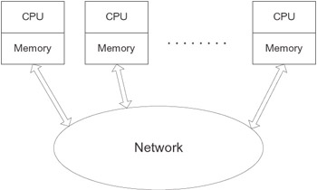
Figure 4.1: Distributed memory multiprocessor.

The primary model of a program for the MPP architecture is parallel processes, each running on a separate processor and using message passing to communicate with each other. There are two main reasons for parallel processes of a message-passing program to send messages among themselves. The first one is that some processes may use data computed by other processes. As this occurs, the data must be delivered from processes producing the data to processes using the data. The second reason is that the processes may need to synchronize their work. Messages are exchanged to inform the processes that some event has happened or some condition has been satisfied.

Since MPPs provide much more parallelism, they have more performance potential than SMPs. Indeed, although the number of processors in SMPs rarely exceeds 32, MPPs often have hundreds and even thousands of processors. Modern communication technologies allow a manufacturer to build such an MPP whose (p + 1)-processor configuration executes “normal” message-passing programs faster than a p-processor configuration for a practically arbitrary p. This means that unlike the SMP architecture, the MPP architecture is scalable.

Many different protocols, devices, physical communications bearers, and the like, may be used to implement communication networks in MPPs. Nonetheless, whatever technical solutions are employed in the particular communication network of an MPP, its main goal is to provide a communication layer that is fast, well balanced with the number and performance of processors, and homogeneous. The structure of the network should cause no degradation in communication speed even when all processors of the MPP simultaneously perform intensive data transfer operations. The network should also ensure the same speed of data transfer between any two processors of the MPP.

The MPP architecture is implemented in the form of parallel computer or in the form of dedicated cluster of workstations. A real MPP implementing the ideal MPP architecture is normally a result of compromise between the cost and quality of its communication network.

To see how the MPP architecture is scalable, consider parallel matrix-matrix multiplication on the ideal MPP. Recall that we have used matrix-matrix multiplication in Chapter 3 to demonstrate that the SMP architecture is not scalable.

The simplest parallel algorithm implementing matrix operation C = A X B on a p-processor MPP, where A, B are dense square n X n matrices, can be summarized as follows:

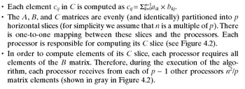
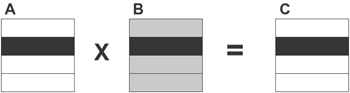
Figure 4.2: Matrix-matrix multiplication with matrices A, B, and C evenly partitioned in one dimension. The slices mapped onto a single processor are shaded in black. During execution, this processor requires all of matrix B (shown shaded in gray).

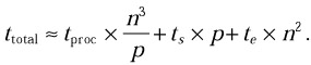
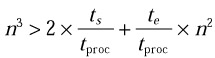
In total, the matrix-matrix multiplication involves O(n³) operations. Therefore the contribution of computation to the total execution time of the parallel

algorithm above is

where t_proc characterizes the speed of a single processor.

To estimate the contribution of communication to the total execution time, assume that the time of transfer of a data block is a linear function of the size of the data block. Thus the cost of transfer of a single horizontal slice between two processors is

where t_s is the start-up time and t_e is the time per element.

During the execution of the algorithm, each processor sends its slice to p - 1 other processors as well as receives their slices. Assume that at any given time the processor can be simultaneously sending a single message and receiving another single message (a double-port model). Then, under the pessimistic assumption that the processor sends its slice to other processors in p - 1 sequential steps, the estimation of the per-processor communication cost is

For simplicity, assume that communications and computations do not overlap. Namely first all of the communications are performed in parallel, and then all of the computations are performed in parallel. So the total execution time of the parallel algorithm on the ideal p-processor MPP is

What restrictions must be satisfied to ensure faster execution of the algorithm on a (p + 1)-processor configuration of the MPP compared with the p-processor configuration (p = 1, 2, . . .)? First of all, the algorithm must ensure speedup at least while upgrading the MPP from a one-processor to a two-processor configuration. It means that

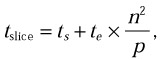
Typically t_s/t_proc ~ 10³ and t_e/t_proc ~ 10¹. Therefore, the inequality

will be comfortably satisfied if n > 100. Second, the algorithm will be scalable, if t_total is a monotonically decreasing function of p, that is, if

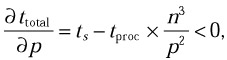
or

The inequality above will be true if n is reasonably larger than p.

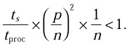
The efficiency of the parallel algorithm above can be significantly improved by using a two-dimensional decomposition of matrices A, B, and C instead of the one-dimensional decomposition. The resulting algorithm of parallel matrix-matrix multiplication can be summarized as follows:

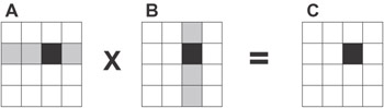
Figure 4.3: Matrix-matrix multiplication with matrices A, B, and C evenly partitioned in two dimensions. The blocks mapped onto a single processor are shaded black. During execution, this processor requires corresponding rows of matrix A and columns of matrix B (shown shaded in gray).

The total per-processor communication cost,

and the total execution time of that parallel algorithm,

are considerably less than in the one-dimensional algorithm. Some further improvements can be made to achieve overlapping communications and computations as well as better locality of computation during execution of the algorithm. As a result the carefully designed two-dimensional algorithm appears efficient and scalable, practically, for any reasonable task size and number of processors.

Summarizing the analysis, we can conclude that the ideal MPP proved to be scalable when executing carefully designed and highly efficient parallel algorithms. In addition, under quite weak, reasonable, and easily satisfied restrictions even very straightforward parallel algorithms make the MPP architecture scalable.

The model of the MPP architecture used in the preceding performance analysis is indeed simplistic. We used three parameters t_proc, t_s, and t_e, and a straightforward linear communication model to describe an MPP. The model was quite satisfactory for the goal of that analysis—to demonstrate the scalability of the MPP architecture. It may also be quite satisfactory for performance analysis of coarse-grained parallel algorithms with simple structure of communications and mainly long messages sent during the communications. However, the accuracy of the model becomes unsatisfactory if one needs to predict performance of a message-passing algorithm with nontrivial communication structure and frequent communication operations transferring mainly short messages, especially if communications prevail over computations.

A more realistic model of the MPP architecture that addresses this issue is the LogP model. It is simple but sufficiently detailed for accurate prediction of the performance of message-passing algorithms with a fine-grained communication structure. In this model the processors communicate by point-to-point short messages. The model specifies the performance characteristics of the interconnection network, but does not describe the structure of the network. The model has four basic parameters:

• L: an upper bound on the latency, or delay, incurred in sending a message from its source processor to its target processor.

• o: the overhead, defined as the length of time that a processor is engaged in the transmission or reception of each message; during this time the processor cannot perform other operations.

• g: the gap between messages, defined as the minimum time interval between consecutive message transmissions or consecutive message receptions at a processor. The reciprocal of g corresponds to the available per-processor communication bandwidth for short messages.

• P: the number of processors.

The model assumes a unit time for local operations and calls it a processor cycle. The parameters L, o, and g are measured as multiples of the processor cycle.

It is assumed that the network has a finite capacity, such that at most L/g messages can be in transit from any processor or to any processor at any time. If a processor attempts to transmit a message that would exceed this limit, it stalls until the message can be sent without exceeding the capacity limit.

The model is asynchronous, that is, processors work asynchronously, and the latency experienced by any message is unpredictable but is bounded above by L in the absence of stalls. Because of variations in latency, the messages directed to a given target processor may not arrive in the same order as they are sent.

The parameters of the LogP model are not equally important in all situations; often it is possible to ignore one or more parameters and work with a simpler model. For example, in algorithms that communicate data infrequently, it is reasonable to ignore the bandwidth and capacity limits. In some algorithms messages are sent in long streams, which are pipelined through the network, so that message transmission time is dominated by the intermessage gaps, and the latency may be disregarded. In some MPPs the overhead dominates the gap, so g can be eliminated.

As an illustration of the role of various parameters of the LogP model, consider the problem of optimal broadcasting a single data unit from one processor to P - 1 others. The main idea is that all processors that have received the data unit transmit it as quickly as possible, while ensuring that no processor receives more than one message.

The source of the broadcast begins transmitting the data unit at time 0. The first data unit enters the network at time o, takes L cycles to arrive at the destination, and is received by the processor at time L + 2 X o. Meanwhile the source will have initiated transmission to other processors at time g, 2 X g,…, assuming g ≥ o, each of which acts as the root of a smaller broadcast tree.

The optimal broadcast tree for p processors is unbalanced with the fan-out at each node determined by the relative values of L, o, and g. Figure 4.4 depicts the optimal broadcast tree for P = 8, L = 6, g = 4, and o = 2. The number shown for each node is the time at which it has received the data unit and can begin sending it on. Notice that the processor overhead of successive transmissions overlaps the delivery of previous messages. Processors may experience idle cycles at the end of the algorithm while the last few messages are in transit.

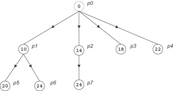
Figure 4.4: Optimal broadcast tree P = 8, L = 6, g = 4, and o = 2. The number shown for each node is the time at which it has received the data unit and can begin sending it.

The algorithm above does no computation. As an example of the usage of the LogP model to analyze a parallel algorithm doing both computation and communication, consider the problem of summation of as many values as possible within a fixed amount of time T. The pattern of communication among the processors again forms a tree. In fact the tree has the same shape as an optimal broadcast tree. Each processor has the task of summing a set of the elements and then (except for the root processor) transmitting the result to its parent. The elements to be summed by a processor consist of original inputs stored in its memory, together with partial results received from its children in the communication tree. To specify the algorithm, first determine the optimal schedule of communication events and then determine the distribution of the initial inputs.

If T ≤ L + 2 X o, the optimal solution is to sum T + 1 values on a single processor, since there is not sufficient time to receive data from another processor. Otherwise, the last step performed by the root processor (at time T - 1) is to add a value it has computed locally to a value it just received from another processor. The remote processor must have sent the value at time T - 1 - L - 2 X o, and we assume recursively that it forms the root of an optimal summation tree with this time bound. The local value must have been produced at time T - 1 - o. Since the root can receive a message every g cycles, its children in the communication tree should complete their summations at times T - (2 X o + L + 1), T - (2 X o + L + 1 + g), T - (2 X o + L + 1 + 2 X g), and so on. The root performs g - o - 1 additions of local input values between messages, as well as the local additions before it receives its first message. This communication schedule must be modified by the following consideration: since a processor invests o cycles in receiving a partial sum from a child, all transmitted partial sums must represent at least o additions. Based on this schedule, it is straightforward to determine the set of input values initially assigned to each processor and the computation schedule. Figure 4.5 shows the communication tree for optimal summing for T = 28, P = 8, L = 5, g = 4, and o = 2.

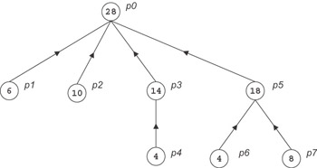
Figure 4.5: Communication tree for optimal summing for T = 28, P = 8, L = 5, g = 4, and o = 2.

The LogP model assumes that all messages are of a small size. A simple extension of the model dealing with longer messages is called the LogGP model. It introduces one more parameter, G, which is the gap per byte for long messages, defined as the time per byte for a long message. The reciprocal of G characterizes the available per-processor communication bandwidth for long messages.

The presented performance models make up a good mathematical basis for designing portable parallel algorithms that run efficiently on a wide range of MPPs via a parametrizing of the algorithms with the parameters of the models. The MPP architecture is much far away from the serial scalar architecture than the vector, superscalar, and SMP architectures. Therefore it is very difficult to automatically generate an efficient message-passing target code for the serial source code written in C or Fortran 77. In fact, optimizing C or Fortran 77 compilers for MPPs would have to solve the problem of automatic synthesis of an efficient message-passing program using the source serial code as a specification of its functional semantics. Although some interesting research results have been obtained in this direction (e.g., during the work on the experimental PARADIGM compiler), they are still far away from practical use. No industrial optimizing C or Fortran 77 compiler for the MPP architecture is available.

Basic programming tools for MPPs are message-passing libraries and high-level parallel languages.