What Is Data Mining?

If data mining is not something akin to magic, just what is it and why should we care? Data mining enables us to put computing power to work, combing through mounds of data to find meaningful bits of information. Data mining takes this number-crunching responsibility out of our hands. We do, however, need to follow a number of steps to prepare the data and the algorithm for the mining process. We also need to evaluate the result to find the gold among the rock produced.

Order from Chaos

Relational database systems are great at piling up mounds of data as they record day-to-day business transactions. Multidimensional systems summarize that data with their aggregations, but they also multiply it along a myriad of dimensions and hierarchies. All this data can be a bit overwhelming. In many cases, this much data is so overwhelming, it is dumped onto backup tapes or placed in archives and forgotten.

The problem, from a business perspective, is that this data is the life story of your organization. It contains the entire record of where your organization has been and, more important, it may be able to provide some clues as to where your organization is going. This information could be helpful in your organization's management. The problem lies in making sense from all this data.

We can compare the task of comprehending these mounds of data with understanding the topography of a patch of land we are preparing to hike across. Each point has a certain elevation above sea level. We could print the elevation of each of these points on our map as shown in Figure 12-1. The result would, indeed, represent the topography of the land, but it would be nearly incomprehensible. This is the same problem we face when we are overwhelmed by transactional and multidimensional data.

	798	799	799	799	799	799	799	800	800	800	800	799	799	799	798	798	798	798	797	797	797	797	797	796
	799	800	800	800	800	800	800	800	803	803	800	800	800	799	798	800	800	800	800	800	800	800	797	796
	799	800	803	805	805	805	805	805	805	805	805	805	805	800	800	805	805	805	805	805	805	803	800	798
	800	801	803	805	808	808	808	808	808	808	808	808	807	805	805	805	808	808	808	807	806	805	802	800
	800	802	804	805	806	809	810	810	810	810	810	810	810	810	810	810	810	810	810	807	805	804	800	800
	800	803	804	805	806	808	810	811	811	812	812	812	812	811	811	811	811	810	808	806	805	803	800	800
	800	800	804	805	806	808	809	810	810	810	810	810	810	810	810	811	811	810	808	806	805	803	800	798
	799	800	803	804	805	806	808	809	809	809	809	809	809	809	809	810	810	810	808	806	805	803	800	798
	799	800	803	804	805	806	807	808	808	808	808	808	808	808	808	809	809	809	807	806	805	803	800	798
	799	800	802	803	804	805	805	806	805	805	805	805	805	805	807	808	808	807	806	806	805	803	800	798
	799	800	802	802	803	804	804	805	804	804	803	803	803	804	805	805	805	805	805	805	805	802	800	798
	799	800	801	801	802	803	804	804	803	803	802	802	802	803	804	804	804	804	804	804	804	802	800	798
	799	799	800	801	802	802	803	803	802	802	801	801	801	802	803	803	803	803	803	803	802	801	800	798
	799	798	799	800	801	801	801	801	800	800	800	800	800	801	802	802	802	802	802	802	802	801	800	798
	798	797	798	799	800	800	800	800	799	799	798	799	799	800	800	801	801	801	801	801	801	801	800	798
	797	879	797	798	799	799	799	799	798	798	797	798	798	799	800	800	800	800	800	800	800	800	800	798

Figure 12-1: Topographic information data overload

Making Connections

In the world of topography, we have the simple, yet powerful, tool of contour lines to help us distill the data down to something understandable. One contour line connects all the points at 800 feet above sea level. Another line connects all the points at 805 feet above sea level. And, yet another, at 810 feet. The remaining values are removed from the map as shown in Figure 12-2.

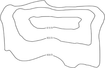
Figure 12-2: A topographic map

The resulting contour map, with its concentric curves, provides almost as much information as the printout of the elevation for every point. The advantage is the contour map is immediately understandable with a little training and experience. With the topographic map, we can plan our route in a matter of minutes, as shown in Figure 12-3, and still have confidence we will not walk off a cliff. With the printout of elevations shown in Figure 12-4, darkness would probably fall before we could figure out which way to go!

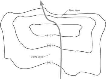
Figure 12-3: Planning a route using a topographic map

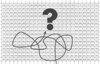
Figure 12-4: Data overload leads to confusion

Data mining works in a manner similar to our topographic map. It makes connections within the data that may not be readily apparent to the human observer. These connections make the data easier to understand. Using this new understanding, we can efficiently analyze the data and set direction, so our organizations do not tumble over a cliff.

Making Predictions

The topographic map holds another advantage for us. Looking at the data shown on the map, we can make predictions of what lies beyond. Judging from the patterns appearing in the contour lines of the map, we can extrapolate to infer the topography of areas beyond the map. This is shown in Figure 12-5.

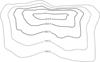
Figure 12-5: Making predictions from the topographic map

With any prediction of the unknown, we have a risk of being incorrect. Still, we have a much better chance of being correct when we work with the patterns provided by the topographic map. Of course, the more data we have to extrapolate from, the better chance we have of making the correct prediction.

Data mining provides us with a similar capability. We can use the patterns found in our data to make predictions of what will happen next. Data mining may find patterns in the way our clients make use of our services. Based on these patterns, we can predict which clients may need additional services in the future. Data mining may find patterns in the valid data entered for a particular screen. Based on these patterns, we can predict whether a newly entered set of data is accurate or contains a data entry error.

Tasks Accomplished by Data Mining

In our topographic map analogy, we touched on a couple of the benefits of data mining. Let's look more specifically at the various tasks data mining can help us accomplish.

Classification

Classification enables us to fit items into slots as shown in Figure 12-6. Perhaps we have a customer we would like to classify as a good credit risk or a bad credit risk. Or, we may need to classify a potential customer as someone who is likely to need our services or someone who is not. If we know how to classify an individual, an entity, or a thing, we can make more intelligent decisions as we deal with that individual, entity, or thing.

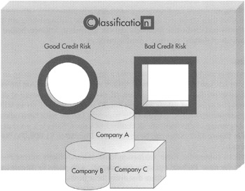
Figure 12-6: Classification

We begin our classification process by selecting the classification we want to make. In other words, we select an attribute whose value we want to predict as part of future transactions. Once we make this selection, we look at the past data. In this data, we already know the value of our prediction attribute. Next, we determine, in the past data, which attributes most distinguish the customers with one value for our prediction attribute from customers with a different value. These distinguishing attributes are then used to forecast the value of the prediction attribute in future transactions.

Let's look at an example. Maximum Miniatures is having a problem with some wholesale customers not paying their invoices in a timely manner. Therefore, we want a way to predict the credit risk of prospective customers. Credit risk is our prediction attribute. We look at the past data, where we already know the value of the credit risk attribute. We know who paid their bills on time and who had to be taken to collections. We can examine the past data and determine the attributes that most distinguish the customers that were good credit risks from those that were bad credit risks. These are the distinguishing attributes. This sounds like an easy thing to do, but if we have millions of records in our past data, it can be a daunting task.

This is where data mining proves its worth. Data mining is excellent at plowing through millions of records to find correlations. It can process the past data and determine whether it is net assets, annual revenue, invoice payment history, or a CEO's favorite color that is a distinguishing attribute for credit risk.

Perhaps customers with over ten million dollars in assets and three million dollars in annual revenue are almost always good credit risks, while customers that don't meet these criteria are almost always bad credit risks. These become our distinguishing attributes: the measures we can apply to prospective customers to determine what their credit risk is likely to be. Using the distinguishing attributes, we can identify bad credit-risk prospects and ask for cash in advance, before they have thousands of dollars' worth of overdue invoices.

Regression

Classification is used to predict the value for a discrete attribute, meaning an attribute that has one of a set number of distinct values. Regression, on the other hand, is used to predict a continuous value. (It would seem the opposite of discrete values would be indiscreet values, but that doesn't sound too good, so we will use the term "continuous values" instead.) The measures that we have been talking about since the beginning of this book are all continuous values. Sales is a good example, as shown in Figure 12-7. Sales can be any number from $0 to $1,000,000,000 (or maybe more).

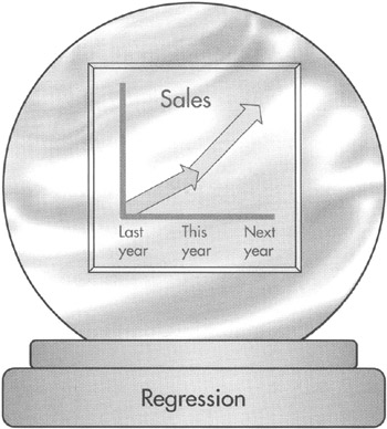
Figure 12-7: Regression

To predict a continuous value, regression looks at trends likely to continue and repeat over time. Perhaps our sales are seasonal, with peaks in August and December. The regression algorithm discovers these peaks while looking at sales figures from past years and continues those trends when predicting future years.

Like classification, regression also looks at relationships between the value being predicted and other continuous values available in the data. In our example, perhaps the price of gasoline has a big effect on sales. (This is certainly true of anyone trying to sell sport utility vehicles!) Our regression algorithm may factor in the price of gasoline at the beginning of the month as it predicts the sales amount for that month.

Segmentation

Segmentation is the "divide and conquer" approach to data analysis. Segmentation divides data into groups with similar characteristics. We can then analyze the characteristics of each group for insights. This is shown in Figure 12-8.

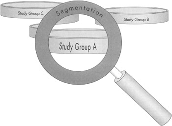
Figure 12-8: Segmentation

For example, a service company can apply segmentation to divide its clients into groups. One group might be companies with over 1,000 employees. Another group might be companies with 500 to 999 employees, and so on. The analyst for the service company can then look at each group to see how much revenue they have generated, what types of needs they have, how much management time they have required, and other factors.

When looking at groups of companies, insights can be gained that would not have been apparent when looking at one company at a time. Using this information, the service company can determine which types of companies should be the focus of its sales and marketing efforts. The service company can also create policies on project management approaches at various types of companies.

Association

Association requires we have some type of grouping in our data. Multiple items could be grouped together in a single sales transaction. Multiple services could be provided to a single family unit. Multiple classes could be taken by a student. This is shown in Figure 12-9.

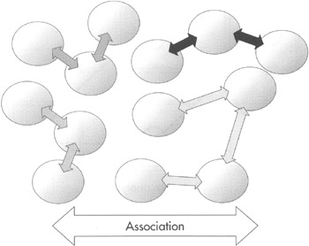
Figure 12-9: Association

The association algorithm examines the groups found in past data to find patterns in the group membership. For example, items A, B, and C may occur together in a large number of groupings. Based on the patterns found, predictions can be made on the makeup of future groups. If items A and B are in a group, there is a strong possibility that item C will be added as well.

We are all familiar with the buying suggestions generated by association. When I have Delivering Business Intelligence with Microsoft SQL Server 2005 from McGraw-Hill/Osborne in my online shopping cart, the website informs me that a number of people who bought this book also purchased Microsoft SQL Server 2005 Reporting Services from McGraw-Hill/Osborne. (How's that for a subtle product plug?)

Classification, segmentation, and association can sometimes run together. They seem similar. The difference is this: With classification, we pick the attribute that defines the grouping and the algorithm determines what most distinguishes those groupings. With segmentation, the algorithm itself creates the grouping, based on what it determines as distinguishing characteristics. With association, the underlying data already contains some type of grouping. The algorithm makes determinations about items likely to be in the group, rather than attributes they are likely to have in common.

Sequence Analysis

Sequence analysis is used to examine ordered stops along a route as shown in Figure 12-10. Data on past routes is processed by the algorithm. Then, the algorithm can predict future routes. Given the current stop, the algorithm can determine the probability of navigating a given route.

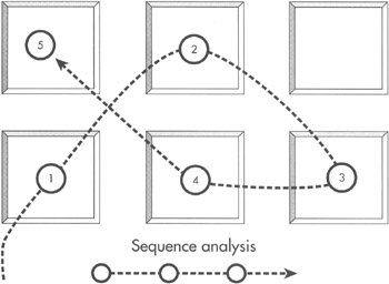
Figure 12-10: Sequence analysis

Sequence analysis is often applied to navigation on a website. A user is on Page A. The user is then most likely to navigate to Page B, with a somewhat smaller probability of navigating to Page C.

Of course, sequence analysis can be applied to other types of events occurring in a sequence. Customers may buy products or utilize services in a particular sequence. We can analyze this data and determine the likely products or services the customer will be interested in next.

Probability Predictions

As stated earlier, data mining is not magic. It cannot see into the future to predict events. Instead, it mathematically analyzes what has occurred in the past and determines what is most probable to occur if present trends continue. A chance always exists that some outside force could cause present trends not to continue. The user, buyer, or prospect we are trying to analyze may be the anomaly that doesn't follow the present trends, even when everyone else does.

At least with data mining, we can determine, with some confidence, what the present trends are. We can then make intelligent decisions based on those trends. Without data mining, we don't know what the trends and associations are, so we are left operating on gut feelings alone.

Steps for Data Mining

Now that you know what data mining can do for you, the next logical question is this: how do I make data mining do all that great stuff for me? Data mining is a multistep process. As with all of the business intelligence approaches we cover in this book, it takes some time and preparation. Despite the complex mathematics data mining algorithms bring to the table, utilizing data mining is not all that complex. This is especially true in SQL Server 2005 and the Business Intelligence Development Studio.

In this section, we introduce the steps required for data mining in the abstract. This lets you gain some familiarity with the general process, without being overwhelmed by the specifics. In Chapter 13, we work through the specific tasks that must be accomplished in the Business Intelligence Development Studio.

Problem Definition

The first step for a data mining solution is to define the problem we are trying to solve. Data mining is great at finding patterns and relationships that are not apparent to human eyes. However, it cannot solve problems unless we point that analytical power in a specific direction.

We need to define the business goal we are working toward. Perhaps we want to do a better job at identifying perspective customers who are a bad credit risk. Perhaps we want to identify customers who are likely to switch to our competitor's products or services. Perhaps we want to predict future sales to put in place the capacity to meet those needs.

Once the business goal is defined, we determine what we need data mining to do for us. We select which of the five data mining tasks we are looking to accomplish:

• Classification

• Regression

• Segmentation

• Association

• Sequence Analysis

Our choice of task influences our choice of data mining algorithm.

SQL Server 2005 provides several algorithms to perform each task. Often, we try several algorithms capable of accomplishing our selected task. We can determine which algorithm proves most accurate for our purpose. We discuss the algorithms provided by SQL Server 2005 and their appropriate tasks in the section "Data Mining Algorithms." With one or more algorithms selected, we determine what data we need to feed into those algorithms.

Data Preparation

When we learned about OLAP cube design, one of our main concerns was where the data to populate the cube was going to come from. With data mining, we have the same concern: where are we going to get the data to be fed into our data mining algorithms?

Data mining in SQL Server 2005 uses the same data sources and data source views we used in our Analysis Services cube projects in the Business Intelligence Development Studio. This gives us great flexibility in where we get our data for data mining. The data source may be tables in a relational database or an OLAP cube in an Analysis Services database. It can also come from one of the OLE DB or other data sources supported by the Business Intelligence Development Studio.

If the data is not readily accessible, we can use the power of SQL Server Integration Services to extract the data, cleanse it, and put it in a location where it can be utilized. You may recall from Chapter 7 a special data flow destination called Data Mining Model Training, which loads data from an Integration Services package directly into a data mining model. We talk about data mining models in Chapter 13.

Training

With algorithms selected and our data in place, we begin the process of working with the data mining model. You can think of a data mining model as the combination of one or more data mining algorithms with some real, live data. The model applies the algorithms to the data and creates the classifications, associations, regression formulas, and so forth that we use to solve our business problem.

This step is known as training the data mining model. We provide our data to the data mining algorithms, so they can be trained on a particular aspect of our organization. They "learn" what is unique about our data, as well as the operations and entities, customers, products, and sales transactions that produced that data.

Validation

We spoke previously in this chapter about providing a data mining algorithm with past data, so it could find the classifications, associations, and so forth contained within. In actuality, we often divide our past data into two sets. One set of data is used to train the data model. The second set is used to validate the model after it is trained. Let's return to our credit risk example for an illustration.

We have historical data containing a number of attributes for our customers, including whether they turned out to be a good credit risk or a bad credit risk. To create and test a data mining model, we divide this data into two sets. One serves to train the model, as we discussed. The second set is used to test each of the data mining algorithms.

The data in the second set is fed into the data mining model and we ask the model to predict which customers will be good credit risks and which will be bad credit risks. Remember, this is historical data, so we already know whether the customers in this set of data were good or bad credit risks.

Each algorithm makes a prediction for each customer in the training data set. Next, we compare the predictions against the known reality for each customer. We can then select the data mining algorithm to use in our production solution based on which had the highest percentage of correct predictions. This algorithm should do the best job of predicting which customers will be good or bad credit risks in the future.

As we separate data into training and testing data sets, it is important we do not do the separation in such a way as to skew the results. For example, taking the first 100,000 records is not a good way to separate the data, especially if we are dealing with transactional records in chronological order. Some event or circumstance may have affected the data during the time the first 100,000 records were generated, which was not present when the rest of the data was generated or as future records are generated. For example, your business may be seasonal. Using a training data set from a time when the seasonal cycle is at its peak can make the data model a poor predictor of outcomes during those times when the cycle is at its nadir.

A random sampling is often a good way to insure impartiality. Data selected from across business cycles can provide the best training for the model. The SQL Server Integration Services row sampling data flow task is excellent for creating random samples for training and testing data mining models.

Deploy

Once we test the data mining model and determine which data mining algorithm gives us the most accurate information, we can put it to work. We place the model where it can be accessed by the front-end tools that will put it to work. We use the Data Mining Extensions (DMX) query language to feed new records to our algorithm and have it generate information. We discuss the DMX query language in Chapter 14.