1.3. Height Field Visualization
| | ||
| | ||
| | ||
1.3. Height Field Visualization
A special area in 3D visualization is the rendering of large terrains , or, more generally , of height fields. A height field is usually given as a uniformly gridded square array h : [0 , N ˆ 1] 2 ![]() , N ˆˆ
, N ˆˆ ![]() , of height values, where N is typically in the order of 16,384 up to several millions. In practice, such a raw height field is often stored in some image file format, such as GIF. A regular grid is, for instance, one of the standard forms in which the US Geological Survey publishes its data, known as the Digital Elevation Model (DEM) [Elassal and Caruso 84].
, of height values, where N is typically in the order of 16,384 up to several millions. In practice, such a raw height field is often stored in some image file format, such as GIF. A regular grid is, for instance, one of the standard forms in which the US Geological Survey publishes its data, known as the Digital Elevation Model (DEM) [Elassal and Caruso 84].
Obviously, a regular grid is not a very efficient data structure, both with regards to memory and rendering. So, alternatively, height fields can be stored as triangular irregular networks (TINs) (see Figure 1.3). They can adapt much better to the detail and features (or lack thereof) in the height field, so they can approximate any surface at any desired level of accuracy with fewer polygons than any other representation [Lindstrom et al. 96]. However, due to their much more complex structure, TINs do not lend themselves to interactive visualization as well as more regular representations.
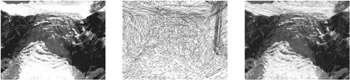
Figure 1.3: A terrain (left), a TIN of its height field (middle), and a superposition (right) [Wahl et al. 04]. (See Color Plate I.)
The problem in terrain visualization is that, if the user looks at it from a low viewpoint directed at the horizon, there are a few parts of the terrain that are very close, while the majority of the visible terrain is at a greater distance. Close parts of the terrain should be rendered with high detail, while distant parts should be rendered with very little detail to maintain a high frame rate.
To solve this problem, a data structure is needed that allows us to quickly determine the desired level of detail in each part of the terrain. Quadtrees are such a data structure, particularly because they seem to be a good compromise between the simplicity of non-hierarchical grids and the good adaptivity of TINs. The general idea is to construct a quadtree over the grid, and then traverse this quadtree top-down in order to render it. At each node, we decide whether the detail offered by rendering it is enough, or if we have to go down further.
One problem with quadtrees (and quadrangle-based data structures in general) is that nodes are not quite independent of each other. Assume we have constructed a quadtree over some terrain, as depicted in Figure 1.4. If we render that as-is, there will be a gap (a crack ) between the top-left square and the fine-detail squares inside the top-right square. The vertices causing this problem are called T-vertices . Triangulating them would help in theory, but in practice, this leads to long and thin triangles that have problems on their own. The solution is to triangulate each node.
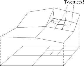
Figure 1.4: In order to use a quadtree for defining a height field mesh, it should be balanced. (Courtesy Prof. R. Klein and R. Wahl, Bonn University.)
Thus, a quadtree offers a recursive subdivision scheme to define a triangulated regular grid (see Figure 1.5): start with a square subdivided into two right-angle triangles; with each recursion step, subdivide the longest side of all triangles (the hypotenuse ), yielding two new right-angle triangles each (hence, this scheme is sometimes referred to as longest edge bisection) [Lindstrom and Pascucci 01]. This yields a mesh where all vertices have degree 4 or 8 (except the border vertices), which is why such a mesh is often called a 4-8 mesh.
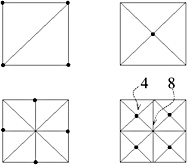
Figure 1.5: A quadtree defines a recursive subdivision scheme yielding a 4-8 mesh. The dots denote the newly added vertices. Some vertices have degree 4, and some have 8 (hence the name ).
This subdivision scheme induces a directed acyclic graph (DAG) on the set of vertices: vertex j is a child of i if it is created by a split of a right angle at vertex i . This will be denoted by an edge ( i, j ). Note that almost all vertices are created twice (see Figure 1.5), so all nodes in the graph have four children and two parents (except the border vertices).
During rendering, we will choose cells of the subdivision at different levels. Let M be the fully subdivided mesh (which corresponds to the original grid) and M be the current, incompletely subdivided mesh. M corresponds to a subset of the DAG of M . The condition of being crack-free can be reformulated in terms of the DAGs associated with M and M :
| (1.1) | 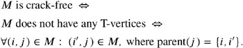 |
In other words: you cannot subdivide one triangle alone; you also must subdivide the one on the other side. During rendering, this means that if you render a vertex, you also have to render all its ancestors (remember that a vertex has two parents).
Rendering such a mesh generates (conceptually) a single, long list of vertices that are then fed into the graphics pipeline as a single triangle strip. The pseudocode for the algorithm looks like this (simplified):
submesh( i , j ) if error( i ) < then return end if if B i outside viewing frustum then return end if submesh( j , c l ) V += p i submesh( j , c r ) where error( i ) is some error measure for vertex i , and B i is the sphere around vertex i that completely encloses all descendant triangles.
Note that this algorithm can produce the same vertex multiple times consecutively; this is easy to check, of course. In order to produce one strip, the algorithm has to copy older vertices to the current front of the list at places where it makes a turn ; again, this is easy to detect, and the interested reader is referred to [Lindstrom and Pascucci 01].
One can speed up the culling a bit by noticing that if B i is completely inside the frustum, we do not need to test the child vertices anymore.
We still need to think about the way we store our terrain subdivision mesh. Eventually, we will want to store it as a single linear array for two reasons:
-
The tree is complete, so it really would not make sense to store it using pointers.
-
We want to map the file that holds the tree into memory as-is (for instance, with the Unix mmap function), so pointers would not work at all.
We should keep in mind, however, that with current architectures, every memory access that cannot be satisfied by the cache is extremely expensive (this is even more so with disk accesses , of course).
The simplest way to organize the terrain vertices is a matrix layout. The disadvantage is that there is no cache locality at all across the major index. To improve this, people often introduce some kind of blocking, where each block is stored in a matrix and all blocks are arranged in matrix order, too. Unfortunately, Lindstrom and Pascucci [Lindstrom and Pascucci 01] report that this is, at least for terrain visualization, worse than the simple matrix layout by a factor 10!
Enter quadtrees. They offer the advantage that vertices on the same level are stored fairly close in memory. The 4-8 subdivision scheme can be viewed as two quadtrees that are interleaved (see Figure 1.6): we start with the first level of the red quadtree that contains just the one vertex in the middle of the grid, which is the one that is generated by the 4-8 subdivision with the first step. Next comes the first level of the blue quadtree that contains four vertices, which are the vertices generated by the second step of the 4-8 subdivision scheme. This process repeats logically. Note that the blue quadtree is exactly like the red one, except it is rotated by 45. When you overlay the red and the blue quadtree, you get exactly the 4-8 mesh.
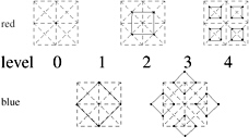
Figure 1.6: The 4-8 subdivision can be generated by two interleaved quadtrees. The solid lines connect siblings that share a common parent. (See Color Plate II.)
Notice that the blue quadtree contains nodes that are outside the terrain grid; we will call these nodes ghost nodes. The nice thing about them is that we can store the red quadtree in place of these ghost nodes (see Figure 1.7). This reduces the number of unused elements in the final linear array down to 33%.
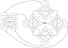
Figure 1.7: The red quadtree can be stored in the unused ghost nodes of the blue quadtree. (See Color Plate III.)
During rendering, we need to calculate the indices of the child vertices, given the three vertices of a triangle. It turns out that by cleverly choosing the indices of the top-level vertices, this can be done as efficiently as with a matrix layout.
The interested reader can find more about this topic in [Lindstrom et al. 96, Lindstrom and Pascucci 01, Balmelli et al. 01, Balmelli et al. 99], and many others.
EAN: N/A
Pages: 69