Color Images

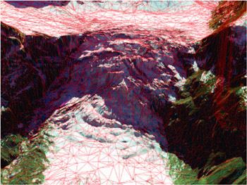
Figure I: A superposition of a terrain and a TIN of its height field [Wahl et al. 04]. (See Figure 1.3.)

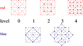
Figure II: The 4-8 subdivision can be generated by two interleaved quadtrees. The solid lines connect siblings that share a common father. (See Figure 1.6.)

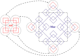
Figure III: The red quadtree can be stored in the unused ghost nodes of the blue quadtree. (See Figure 1.7.)

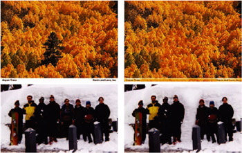
Figure IV: Some results of the texture synthesis algorithm [Wei and Levoy 00]. In each pair, the image on the left is the original one, the one on the right is the (partly) synthesized one. (See Figure 2.14.)

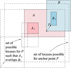
Figure V: By estimating the volume of the Minkowski sum of two BVs, we can derive an estimate for the cost of the split of a set of polygons associated with a node. (See Figure 4.8.)

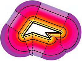
Figure VI: Example of a distance field in the plane for a simple polygon (thick black lines). The distance field inside the polygon is not shown. The dashed lines show the Voronoi diagram for the same polygon. The thin lines show isosurfaces for various isovalues. (See Figure 5.1.)

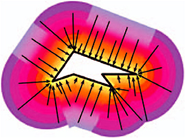
Figure VII: The vector distance field for the same polygon as shown on the left. Only a few vectors are shown, although (in theory) every point of the field has a vector. (See Figure 5.2.)

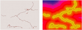
Figure VIII: A network of roads described in the plane by a set of edges (left) and the distance map of these roads . The distance of each point in the plane from a road is color -coded. It could be used, for example, to determine the areas where new houses can be built. (See Figure 5.3.)

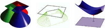
Figure IX: (left) The distance function of a point site in the plane is a cone. (middle) More complex sites have a bit more complex distance functions. (right) The distance function of sites in 3D is different for the different slices of the volume [Hoff III et al. 99]. (See Figure 5.6.) (Courtesy of K. Hoff, T. Culver, J. Keyser, M. Lin, and D. Manocha, Copyright ACM.)

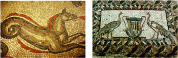
Figure X: Roman mosaics from baths [Mosaic a, Mosaic b]. See Figure 6.26.)

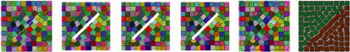
Figure XI: Process to preserve edges of the original image in the final mosaic. [Hausner 01]. (See Figure 6.31.)

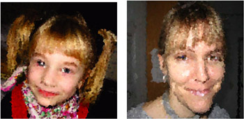
Figure XII: Mosaics generated by randomly placing 6000 Voronoi sites on an image and coloring each Voronoi region uniformly by the color in the image. (See Figure 6.32.)

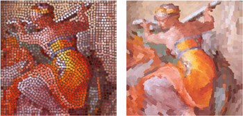
Figure XIII: Two examples of mosaics [Hausner 01], generated with the CVD method. (See Figure 6.33.)

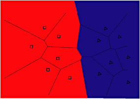
Figure XIV: Conceptually, the nearest -neighbor classifier partitions the feature space into Voronoi cells . (See Figure 7.14.)

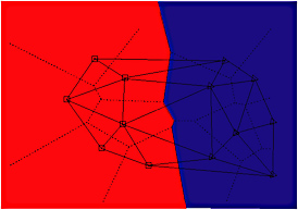
Figure XV: The decision boundary of the nearest-neighbor classifier runs between Delaunay neighbors with different colors. (See Figure 7.15.)

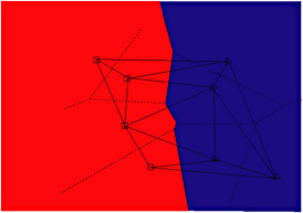
Figure XVI: The edited training set has the same decision boundary, but fewer nodes. (See Figure 7.16.)

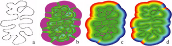
Figure XVII: Visualization of the implicit function f(x) over a 2D point cloud. Points x ˆˆ ² with f(x) ‰ˆ 0, i.e., points on or close to the surface, are shown magenta . Red denotes f(x) ‰ 0, and blue denotes f(x) ‰ 0. (a) point cloud; (b) reconstructed surface using the definition of [Adamson and Alexa 03]; (c) utilizing the centered covariance matrix produces a better surface, but it still has several artifacts; (d) surface and function f(x) based on the SIG. (See Figure 7.21.)

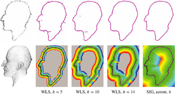
Figure XVIII: Reconstructed surface based on simple WLS and with proximity graph (rightmost) for a noisy point cloud obtained from the 3D Max Planck model (leftmost). Notice how fine details, as well as sparsely sampled areas, are handled without manual tuning. (See Figure 7.23.)

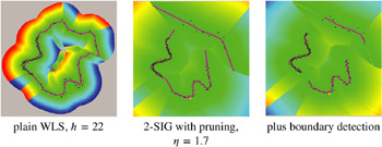
Figure XIX: Automatic sampling density estimation for each point allows you to determine the bandwidth automatically and independently of scale and sampling density (middle), and to detect boundaries automatically (right). (See Figure 7.24.)

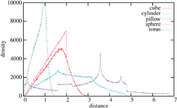
Figure XX: The shape distributions of a number of different simple objects. (See Figure 2.15.)

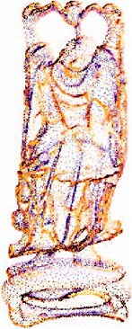
Figure XXI: One of the test objects for Figure 7.30. (See Figure 7.31.)