7.4. Intersection Detection between Point Clouds

The surface defintion described in the previous sections is well suited for quick rendering, for instance, by ray tracing. In addition, it can also be used to determine the intersection between two point-cloud objects [Klein and Zachmann 05]. This will be explained in the following sections.

The problem is the following. Given two point clouds A and B , the goal is to determine whether there is an intersection, i. e., a common root f _A ( x ) = f _B ( x ) = 0, and, possibly, to compute a sampling of the intersection curve(s), i. e., of the set = { x f _A ( x ) = f _B ( x ) = 0}.

In principle, one could just use one of the many general root-finding algorithms [Pauly et al. 03, Press et al. 92]. However, finding common roots of two (or more) non-linear functions is extremely difficult. Even more so here, because the functions are not described analytically, but algorithmically.

Fortunately, here we can exploit the proximity graph we already have in the surface definition of the objects and, thus, achieve much better performance.

First, the algorithm tries to bracket intersections by two points on one surface and on either side of the other surface (see Figure 7.25). Second, for each such bracket , it finds an approximate point in one of the point clouds that is close to the intersection (see Figure 7.26). Finally, this approximate intersection point is refined by subsequent randomized sampling. This last step is optional, depending on the accuracy needed by the application.

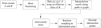
Figure 7.25: Outline of the point-cloud intersection detection.

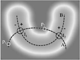
Figure 7.26: Two point clouds A and B and their intersection spheres I ₁ and I ₂ .The root-finding procedure, when initialized with p ₁ , p ₂ ˆˆ A, will find an approximate intersection point inside the intersection sphere I ₁ .

Steps 1 and 3 will be solved by a randomization approach. Both steps 1 and 2 will utilize the proximity graph. In the following, we describe each step in detail.

7.4.1. Root Bracketing

As mentioned earlier, the algorithm starts by constructing random pairs of points on different sides of one of the surfaces. The two points should not be too far apart, and the pairs should evenly sample the surface.

An exhaustive enumeration of all pairs is, of course, prohibitively expensive. Therefore, we pursue the following randomized (sub-)sampling procedure.

Assume that the implicit surface is conceptually(!) approximated by surfels (2D discs) of equal size [Pfister et al. 00, Rusinkiewicz and Levoy 00]. Let Box( A, B ) = Box( A ) ˆ Box( B ) and A = A ˆ Box( A, B ). Then we want to randomly draw points p _i ˆˆ A such that each surfel s _i gets occupied by at least one p _i ; here, occupied by p _i means that the projection of a ( p _i ) along the normal n ( p _i ) onto the supporting plane of s _i lies within the surfels radius.

For each p _i , we can easily determine another point p _j ˆˆ A in the neighborhood of p _i (if any), so that p _i and p _j lie on different sides of f _B . We represent the neighborhood of a point p _i by a sphere C _i centered at p _i .

An advantage of this approach is that the application can specify the density of the intersection points that are to be returned by our algorithm. From these, it is fairly easy to construct a discretization of the complete intersection curves (e. g., by using randomized sampling again).

Note that we never need to actually construct the surfels or assign the points from A explicitly to the neighborhoods, which we describe in the following. Section 7.4.2 describes how to choose the radius of the spheres C _i .

In order to find a p _j ˆˆ A ˆ C _i on the other side of f _B , we use f _B ( p _i ) f _B ( p _j ) ‰ 0 as an indicator. This, of course, is reliable only if the normals n ( x ) are consistent throughout space. If the surface is manifold , this can be achieved by a method similar to [Hoppe et al. 92]: utilizing a proximity graph (such as the SIG), we can propagate a normal to each point p _i ˆˆ A . Then, when defining f ( x ), we choose the direction of n ( x ) according to the normal stored with the nearest neighbor of x . ^[6]

In order to sample A such that each (conceptual) surfel is represented by at least one point in the sample, we use the following.

Lemma 7.4. Let A be a uniformly sampled point cloud. Further, let S _A denote the set of conceptual surfels approximating the surface of A inside the intersection volume of A and B, and let a = S _A . Then we can occupy each surfel with at least one point with probability , where c is an arbitrary constant, just by drawing n = O ( a ln a + c a ) random and independent points from A . These points will be denoted as A .

Proof: see [Klein and Zachmann 05].

For instance, if we want p ‰ 97%, we must choose c = 3 . 5, and if a = 30, then we must draw n ‰ˆ 200 random points.

The next section will show how to choose an appropriate size for the neighborhoods C _i . After that, Section 7.4.3 will propose an efficient way to determine the other part p _j of the root brackets given a point p _i ˆˆ A .

7.4.2. Size of Neighborhoods

The radius of the spherical neighborhoods C _i must be chosen so that, on the one hand, all C _i cover the whole surface defined by A . On the other hand, the intersection with each adjoining neighborhood of C _i has to contain at least one point in A so as to not miss any collisions lying in the intersection of two neighborhoods. The situation is illustrated in Figure 7.27.

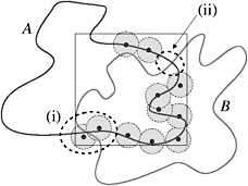
Figure 7.27: If the spherical neighborhoods C _i (filled disks) are too small, not all collisions can be found. (i) Adjoining neighborhoods might not overlap sufficiently, so their intersection contains no randomly chosen cloud point. (ii) The surface might not be covered by neighborhoods C _i .

To determine the minimal radius of a spherical neighborhood C _i , we introduce the notion of sampling radius .

Definition 7.5. (Sampling radius.) Let a point cloud A as well as a subset A A be given. Consider a set of spheres, centered at A , that cover the surface defined by A (not A ), where all spheres have equal radius. We define the sampling radius r ( A ) as the minimal radius of such a sphere covering.

The sampling radius r ( A ) can obviously be estimated as the radius r of a surfel s _i ˆˆ S _A .

Let F _A denote the surface area of the implicit surface over A . Then the surfel radius r can be determined by

Assume that the implicit surface over A can also be approximated by surfels of size r ( A ). Then, F _A can be estimated by

Overall, r ( A ) can be estimated by

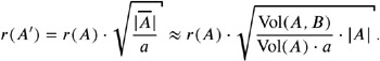
The size of A , A , can easily be estimated as , and the sampling radius r ( A ) can easily be determined in the preprocessing.

7.4.3. Completing the Brackets

Given a point p _i ˆˆ A , we need to determine other points p _j ˆˆ A ˆ C _i on the other side of f _B in order to bracket the intersections. From a theoretical point of view, this could be done by testing f _B ( p _i ) f _B ( p _j ) ‰ 0 for all points p _j ˆˆ A ˆ C _i in time O (1) because A can be a chosen constant. In practice, however, the set A ˆ C _i cannot be determined quickly. Therefore, in the following, we propose an adequate alternative that works in time O (log log N ).

We observe that A ˆ C _i ‰ˆ A ˆ A _i , where A _i := { x 2 r ( A ) ˆ ‰ x ˆ p _i ‰ 2 r ( A )} is an anulus around p _i (or, at least, these are the p _j that we need to consider to ensure a certain bracket density). By construction of A , A ˆ A _i has a similar distribution as A ˆ A _i . Observe further, that we dont necessarily need p _j ˆˆ A .

Overall, the idea is to construct a random sample B _i A ˆ C _i such that B _i A _i , B _i ‰ˆ A ˆ A _i , and such that B _i has a similar distribution as A ˆ A _i.

This sample B _i can be constructed quickly by the help of Lemma 7.4. We just choose randomly O ( b ln b ) many points from A ˆ A _i , where b := A ˆ C _i .

We can describe the set A ˆ A _i very quickly if the points in the CPSP (close-pairs shortest- path ) map stored with p _i are sorted by their geodesic ^[7] distance from p _i . Then we just need to use interpolation search to find the first point with distance 2 r ( A ) ˆ and the last point with distance 2 r ( A ) from p _i. This can be done in time O (log log A ˆ C _i ) per point p _i ˆˆ A . Thus, the overall time to construct all brackets is in O (log log N ).

7.4.4. Interpolation Search

Having determined two points p ₁ , p ₂ ˆˆ A on different sides of surface B , the next goal is to find a point ˆˆ A between p ₁ and p ₂ that is as close as possible to B . In the following, we will call such a point the approximate intersection point (AIP). The true intersection curve f _B ( x ) = f _A ( x ) = 0 will pass close to (usually, it does not pass through any points of the point clouds).

Depending on the application, might already suffice. If the true intersection points are needed, then we refine the output of the interpolation search by the procedure described in Section 7.4.6.

Here, we can exploit the proximity graph. We just consider the points P ₁₂ that are on the shortest path between p ₁ and p ₂ , and we look for that assumes .

Let us assume that f _B is monotonic along the path p ₁ p ₂ . Then, instead of doing an exhaustive search along the path, we can utilize interpolation search to look for with f ( ) = 0. ^[8] This makes sense here, because the access to the key of an element, i. e., an evaluation of f _B ( x ), is fairly expensive [Sedgewick 89]. The average runtime of the interpolation search is in O (log log m ), m = number of elements.

Algorithm 7.5 for the interpolation search assumes that the shortest paths are precomputed and stored in a map.

However, in practice, the memory consumption, albeit linear, could be too large for huge point clouds. In that case, we can compute the path P on the fly at runtime by Algorithm 7.6. Theoretically, the overall algorithm is now in linear time. However, in practice, it still behaves sublinearly because the reconstruction of the path is negligible compared to evaluating f _B .

If f _B is not monotonic along the paths between the brackets, but the sign of f _B ( x ) is consistent, then we can use a binary search to find . (The complexity in that case is O (log m ).)

Algorithm 7.5: Pseudocode for the root-finding algorithm based on interpolation search. P is an array containing the points of the shortest path from p ₁ = P ₁ to p ₂ = P _n , which can be precomputed. d _i = f _B (P _i ) approximates the distance of P _i to object B. (*) Note that either d _l or d _r is negative.

  l, r  = 1  , n   d  _l,r =  f  _B (  P  ₁ )  , f  _B (  P  _n )  while   d  _l  >       and  d  _r  >       and  l   < r   do        d  _x =  f  _B (  P  _x )  if   d  _x  <   then   l, r  =  x, r   else   l, r  =  l, x   end if   end while

Algorithm 7.6: This algorithm can be used to initialize P for Algorithm 7.5 if precomputing and storing all shortest paths in a map is too expensive. (q is a priority queue.)

  q  .insert(  p  ₁ ); clear  P   repeat   p  =  q  .pop  P  .append(  p  )  for all   p  _i adjacent to  p   do   if   d  _geo (  p  _i  , p  ₂ )  < d  _geo (  p  ₁  , p  ₂ )  then  insert  p  _i into  q  with priority  d  _geo (  p  _i  , p  ₂ )  end if   end for   until   p  =  p  ₂

7.4.5. Models with Boundaries

If the models have boundaries and the sampling rate of the root-bracketing algorithm is too low, not all intersections will be found (see Figure 7.28). In that case, some AIPs might not be reached, because they are not connected through the proximity graph.

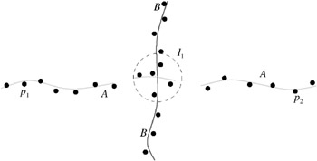
Figure 7.28: Models with boundaries can cause errors (I ₁ could remain undetected), which can be avoided by virtual edges in the proximity graph.

Therefore, we modify the r -SIG a bit for our purpose. After constructing the graph, we usually prune away all long edges by an outlier detection algorithm (see Section 7.1.2). Now, we only mark these edges as virtual. Thus, we can still use the r -SIG for defining the surface as before. For our interpolation search, however, we can also use the virtual edges so that small holes in the model are bridged.

7.4.6. Precise Intersection Points

If two point clouds are intersecting, the interpolation search computes a set of AIPs. Around each of them, an intersection sphere of radius r = min( x ˆ ₁ , x ˆ ₂ ) contains a true intersection point, where

the _i have been computed by the interpolation search, lying on different sides of surface B , and d _i = f _B ( p _i ). This idea is illustrated in Figure 7.29. So if the AIPs are not precise enough, we can sample each such sphere to get more accurate (discrete) intersection points.

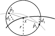
Figure 7.29: An intersection sphere centered at an AIP p _i . Its radius r can be determined approximately with the help of a second point on the other side of B.

More precisely, if we want a precise collision points distance from the surfaces to be smaller than _2, we cover a given intersection sphere by s smaller spheres with diameter ₂ and sample that volume by s ln s + cs many points so that each of the s spheres gets a point with high probability. For each of these, we just determine the distance to both surfaces.

[Rogers 63] showed that a sphere with radius a b can be covered by at most smaller spheres of radius b . Since we would like to cover the intersection sphere by spheres with radius b = ₂ /2, we need to choose a = 2 r / ₂ , so that a b = r . As a consequence,

For example, to cover an intersection sphere with spheres of radius , then ₂ = 2 and .

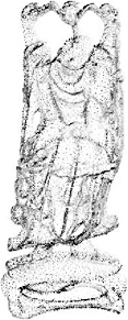
Figure 7.31: One of the test objects for Figure 7.30. (See Color Plate XXI.)

7.4.7. Running Time

Under some mild assumptions about the point cloud, the running time of the algorithm is in O (log log N ), where N is the number of points [Klein and Zachmann 05].

Empirically, it was found that about n = O ( a ln a ) = 200 samples in phase 1 of the algorithm yields a sufficient bracket density so that the error is only about 0.1%.

The performance of a simple implementation in C++, running on a 2.8 GHz Intel Pentium IV, for detecting all intersections between two objects, depending on different densities of the point clouds, is shown in Figure 7.30. (We define the density of an object A with N points as the ratio of N over the number of volume units of the AABB of A , which is at most 8, as each object is scaled uniformly so that it fits into a cube of size 2 ³ . Computing the shortest paths between ( p _i , p _j )on the fly during interpolation search (see Algorithm 7.6) incurs at most an additional 10% of the overall running time.

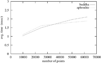
Figure 7.30: The plot shows the running time depending on the size of the point clouds for two objects (see Figures 7.19 and 7.31). The time is the average of all intersection detection times for distances between 0 and 1.5 and a lot of different orientations for two identical copies of each object.

^[6] Surprisingly, the direction of n ( x ) is consistent over fairly large volumes without any preconditioning.

^[7] By using the geodesic distance (or, rather, the approximation thereof), we basically impose a different topology on the space where A is embedded, but this is actually desirable.

^[8] In practice, the interpolation search will never find exactly such a , but instead a pair of adjacent points on the path that straddle B .