4.3. Collision Detection

Fast and exact collision detection of polygonal objects undergoing rigid motions is at the core of many simulation algorithms in computer graphics. In particular, all kinds of highly interactive applications such as virtual prototyping need exact collision detection at interactive speeds for very complex, arbitrary polygon soups. It is a fundamental problem of dynamic simulation of rigid bodies, simulation of natural interaction with objects, and haptic rendering.

BVHs seem to be a very efficient data structure to tackle the problem of collision detection for rigid bodies. All kinds of different types of BVs have been explored in the past: sphere [Hubbard 95, Palmer and Grimsdale 95], OBBs [Gottschalk et al. 96], DOPs [Klosowski et al. 98, Zachmann 98], AABBs [Zachmann 97, van den Bergen 97, Larsson and Akenine-Mller 01], and convex hulls [Ehmann and Lin 01], to name but a few.

Algorithm 4.2: General scheme of hierarchical collision detection.

   traverse(A,B)    if  A and B do not overlap  then   return   end if   if  A and B are leaves  then   return  intersection of primitives                        enclosed by A and B  else   for all  children A[i] and B[j]  do  traverse(A[i],B[j])  end for   end if

Given two hierarchical BV data structures for two objects A and B , almost all hierarchical collision detection algorithms implement the general scheme shown in Algorithm 4.2. This algorithm is essentially a simultaneous traversal of two hierarchies, which induces a so-called bounding volume test tree (BVTT) (see Figure 4.12). Each node in this tree denotes a BV overlap test. Leaves in the BVTT denote an intersection test of the enclosed primitives (polygons); whether or not a BV test is done at the leaves depends on how expensive it is compared to the intersection test of primitives.

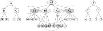
Figure 4.12: The bounding volume test tree is induced by the simultaneous traversal of two BVHs. ( Courtesy of the editors of the Proceedings of Vision, Modeling, and Visualization 2003.)

The characteristics of different hierarchical collision detection algorithms lie in the type of BV used, the overlap test for a pair of nodes, and the algorithm for construction of the BVHs.

During collision detection, the simultaneous traversal will stop at some nodes in the BVTT. Let us call the set of nodes, of which some children are not visited (because their bounding volumes do not overlap), the bottom slice through the BVTT (see the curved lines in Figure 4.12).

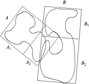
Figure 4.11: Hierarchical collision detection can discard many pairs of polygons with one bounding volume check. Here, all pairs of polygons from A ₁ and B ₂ can be discarded.

One idea is to save this set for a given pair of objects [Li and Chen 98]. When this pair is to be checked next time, we can start from this set, going either up or down. If the objects have moved only a little relative to each other, the number of nodes that need to be added or removed from the bottom slice should be small. This scheme is called incremental hierarchical collision detection .

4.3.1. Stochastic Collision Detection

It has often been noted that the perceived quality of a virtual environment (and, in fact, most interactive 3D applications) crucially depends on the real-time response to collisions [Uno and Slater 97]. It depends much less on the correctness of the simulation, because humans cannot distinguish between physically correct and physically plausible behavior of objects (at least to some degree) [Barzel et al. 96]. ^[5]

Therefore, we can exploit this to develop an inexact collision detection method [Klein and Zachmann 03]. The benefit is that the algorithm is time-critical, i. e., the application can control the running time by pre-specifying the desired quality or a certain time budget for the collision detection.

The idea is a fairly simple average-case approach : conceptually, the main idea of the new algorithm is to consider sets of polygons at inner nodes of the BVH. Then, during traversal, for a given pair of BVH nodes, we not only check the bounding volumes for overlap, but also try to estimate the probability that the two sets of polygons intersect.

Algorithm 4.3: Time-critical traversal scheme. The recursive procedure is now replaced by a queue.

   traverse    (    A, B    )   while   q  is not empty  do   A, B     q  .pop  for  all children  A  _i and  B  _j  do   p     P  [  A  _i  , B  _j ]  if   P  [  A  _i  , B  _j ] is large enough  then   return  collision  else if   P  [  A  _i  , B  _j ]  >   then   q  .insert(  A  _i  , B  _j  , P  [  A  _i  , B  _j ])  end if   end for   end while

Since the exact order in which nodes in the BVTT (see Figure 4.12) are visited is unimportant, we can change the traversal scheme from above and direct the traversal first into those subtrees where a collision is more likely. Thus, the time-critical traversal scheme for two BVHs looks like Algorithm 4.3, where P [ A _i , B _j ] denotes the probability that there is an intersection between the polygons enclosed by A _i and B _j , and q is a priority queue, which is initialized with the root bounding volume pair.

In the following, we will see how to estimate the probability of intersection between two BVs without ever checking any polygons (until we reach the leaves) and without storing any polygons at inner nodes.

Let us first begin with a simple thought experiment ( Gedankenexperiment ). Consider a simple cell in space, for instance, a cube (see Figure 4.13, left image). Assume we know that this cell contains a polygon from object A with maximal surface area such that it just fits completely inside the cell. Assume further that we also have a similar maximal polygon from object B inside the cell. Then we know, without further computation, that there must be an intersection between objects A and B .

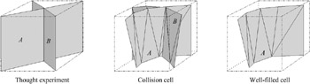
Figure 4.13: Left: thought experiment illustrating our approach to estimate the probability of an intersection between the surfaces contained a pair of bounding volumes during traversal. Middle: practical case, defined as collision cell. Right: definition of a well-filled cell.

In practice, of course, we never have such maximal polygons. What does happen, though, is that a part of the surface of A is inside the cell that has the same area as the maximal polygon from the thought experiment, and also a similar part of B (see Figure 4.13, middle image). In that case, a collision is at least very likely. We define that case as a collision cell .

Conceptually, given a pair of bounding volumes ( A, B ) (for sake of illustration we use AABBs), we determine the probability of an intersection as follows (see Figure 4.14):

Partition A ˆ B into a regular grid;
Determine the cells that are well-filled by polygons from A (see Figure 4.13, right image);
Determine cells well-filled from B ;
Count the number c ( A ˆ B ) of collision cells, i. e., cells that are well-filled by A and B .

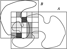
Figure 4.14: The (conceptual) idea of the time-critical collision detection method is to count the number of cells that are well-filled by polygons from A and from B. (Courtesy of Blackwell Publishing.)

It is well understood that this method would be much too slow. Therefore, we dont actually count the number c , but rather estimate it as follows.

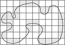
Figure 4.15: During BVH construction, we determine the overall number of cells inside bounding volume A that are well-filled.

During BVH construction (which is preprocessing), we partition each BV by a grid and count the number, s _A , of well-filled cells. This number is stored with the node in the BVH. At runtime, we estimate the number of well-filled cells in the volume A ˆ B as

and, similarly, we estimate .

Now, we reduce the estimation of P [ A, B ], the probability that there is an intersection, to the estimation of the probability that there are at least x many collision cells, P [ c ( A ˆ B ) ‰ x ], by a combinatorial argument.

This probability can be computed quite easily by the so-called balls-into- bins model : given a number of bins, s , and a number of light balls, s _A , and dark balls, s _B , we throw the balls randomly into the bins, with the additional constraint that each bin may contain at most one light and one dark ball (see Figure 4.16).

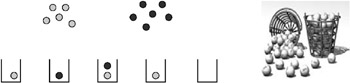
Figure 4.16: The balls-into-bins model. (Right image courtesy of Animation Factory.)

Using this model, the probability that there are c ‰ x collision cells ( x < s _A , s _B ) is

(4.16)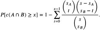

Note that we assume that the well-filled cells in each bounding volume are evenly distributed.

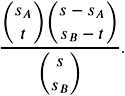
Proof: Let us assume the s _A light balls have already been thrown into the bins. Without loss of generality, we can assume that the first s _A bins are occupied by one light ball each. The overall number of possibilities to distribute the s _B dark balls into the s bins is . However, the number of possibilities that exactly t of the s _B dark balls fall into a light bin is , because there are many possibilities to pick exactly t light bins and many possibilities to pick exactly s _B ˆ t unoccupied bins. Applying the rule number of favorable divided by number of overall possibilities, it is easy to see that the probability that exactly t bins get a dark and a light ball is

Obviously, P decreases and the likelihood for an intersection increases as x increases.

The good thing now is that we can precompute a look-up table for P . We can partition each BV in the BVH by, say, 8 ³ grid cells, so that s, s _A , s _B ˆˆ [0 , 512]. Exploiting symmetry and the monotonicity of P , such a look-up table uses on the order of 10 to 30 MB. For the details, we refer you to [Klein and Zachmann 03].

Note that this approach is a general framework that can be applied to many BVHs with different types of BVs. The BVH must be augmented by a single number: the number of cells in each node that contain many polygons. ^[6]

Figure 4.17 shows an example of an implementation with AABB trees, demonstrating how the running time can be influenced by the probability threshold and how the error changes accordingly .

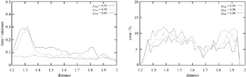
Figure 4.17: Running time (left) and error (right) of an example implementation of time-critical collision detection. (Objects: two copies of a car body, 60,000 polygons each.)

^[5] Analogously to rendering, a number of human factors determine whether or not the incorrectness of a simulation will be noticed. These include the mental load of the viewing person, cluttering of the scene, occlusions, velocity of the objects and the viewpoint, point of attention, etc.

^[6] One could even discard the polygons altogether, if one never wants to perform exact collision detection. In that case, we could just say that there is a collision if the probability computed at a pair of leaves is above a threshold.