Nice, Colorful, Impressive, and Dynamic Graphs

Creating a chart from the data you have just entered is really pretty easy. Start by selecting the cells that represent the information you want to see on your finished chart, including the headings. You can start with one corner of the chart and simply drag your mouse across to select all that you want. Using the spreadsheet we created, select the area that includes cell A4 through to F9. Note that I did not include row 11, the totals line.

Warning

If there are some empty cells in your table (in my example, row 5), you need to deselect them. You can do this by holding down the <Ctrl> key and clicking those cells with the mouse.

After you have all the cells you want selected, click Insert on the menu bar, and select Chart. This window gives you the opportunity of assigning certain rows and columns as labels (see Figure 14-7). This is perfect because we have the quarter numbers running down the left side and the year labels running across the top. Check these on.

Figure 14-7. The AutoFormat Chart dialog.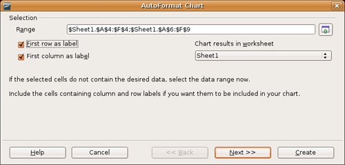

Before you move on, notice the Chart Results in Worksheet drop-down list. By default, Calc creates three tabbed pages for every new worksheet, even though you are working on only one at this time. If you leave things as they are, your chart is embedded into your current page, though you can always move it to different locations. At this point, you have a choice to have the chart appear on a separate page (see those tabs at the bottom of your worksheet). For my example, I'm going to leave the chart on the first page. Make your selection, and then click Next.

Note

There is also an Insert Chart icon on the Standard bar. If you click that icon (instead of clicking Insert and then Chart from the menu bar), the software automatically assumes that you want the chart in the worksheet. Furthermore, your cursor changes to a small chart icon. Click a location on the document where you want the chart to appear and the AutoFormat Chart dialog appears.

The next window lets you choose from chart types (bar, pie, and so on) and provides a preview window to the left (see Figure 14-8). That way, you can try the various chart options to see what best shows off your data. If you want to see the labels in your preview window, click the check box for Show Text Elements in Preview.

Figure 14-8. Lots of chart types to choose from.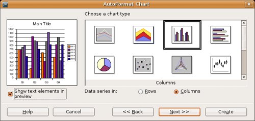

You can continue to click Next for some additional fine-tuning on formatting (the last screen lets you change the title), but this is all the data you need to create your chart. When you are done, click the Create button, and your chart appears on your page (see Figure 14-9).

Figure 14-9. Just like that, your chart appears alongside your table.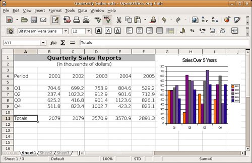

To lock the chart in place, click anywhere else on the worksheet. You may want to change the chart's title, as well; double-click the chart, then click the title to make your changes. I'm going to call mine Sales Over 5 Years. If the chart is in the wrong place, click it, then drag it to where you want it to be. If it is too big, grab one of the corners and resize it.

What's cool about this chart is that it is dynamically linked to the data on the page. Change the data in a cell, press <Enter>, and the chart automatically updates!