2. Full-Reference Quality Assessment using Error Sensitivity Measures

2. Full-Reference Quality Assessment using Error Sensitivity Measures

An image or video signal whose quality is being evaluated can be thought of as a sum of a perfect reference signal and an error signal. We may assume that the loss of quality is directly related to the strength of the error signal. Therefore, a natural way to assess the quality of an image is to quantify the error between the distorted signal and the reference signal, which is fully available in FR quality assessment. The simplest implementation of the concept is the MSE as given in (1). However, there are a number of reasons why MSE may not correlate well with the human perception of quality:

1. Digital pixel values on which the MSE is typically computed, may not exactly represent the light stimulus entering the eye.

2. The sensitivity of the HVS to the errors may be different for different types of errors, and may also vary with visual context. This difference may not be captured adequately by the MSE.

3. Two distorted image signals with the same amount of error energy may have very different types of errors.

4. Simple error summation, like the one implemented in the MSE formulation, may be markedly different from the way the HVS and the brain arrives at an assessment of the perceived distortion.

In the last three decades, most of the proposed image and video quality metrics have tried to improve upon the MSE by addressing the above issues. They have followed an error sensitivity based paradigm, which attempts to analyze and quantify the error signal in a way that simulates the characteristics of human visual error perception. Pioneering work in this area was done by Mannos and Sakrison [12], and has been extended by other researchers over the years. We shall briefly describe several of these approaches in this section. But first, a brief introduction to the relevant physiological and psychophysical components of the HVS will aid in the understanding of the algorithms better.

2.1 The Human Visual System

Figure 41.1 schematically shows the early stages of the HVS. It is not clearly understood how the human brain extracts higher-level cognitive information from the visual stimulus in the later stages of vision, but the components of the HVS depicted in Figure 41.1 are fairly well understood and accepted by the vision science community. A more detailed description of the HVS may be found in [13–15].

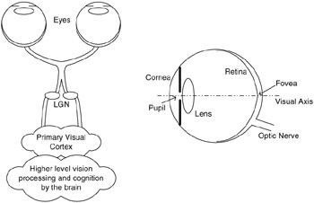
Figure 41.1: Schematic diagram of the human visual system.

2.1.1 Anatomy of the HVS

The visual stimulus in the form of light coming from objects in the environment is focussed by the optical components of the eye onto the retina, a membrane at the back of the eyes that contains several layers of neurons, including photoreceptor cells. The optics consists of the cornea, the pupil (the aperture that controls the amount of light entering the eye), the lens and the fluids that fill the eye. The optical system focuses the visual stimulus onto the retina, but in doing so blurs the image due to the inherent limitations and imperfections. The blur is low-pass, typically modelled as a linear space-invariant system characterized by a point spread function (PSF). Photoreceptor cells in the retina sample the image that is projected onto it.

There are two types of photoreceptor cells in the retina: the cone cells and the rod cells. The cones are responsible for vision in normal light conditions, while the rods are responsible for vision in very low light conditions, and hence are generally ignored in the modelling. There are three different types of cones, corresponding to three different light wavelengths to which they are most sensitive. The L-cones, M-cones and S-cones (corresponding to the Long, Medium and Short wavelengths at which their respective sensitivities peak) split the image projected onto the retina into three visual streams. These visual streams can be thought of as the Red, Green and Blue color components of the visual stimulus, though the approximation is crude. The signals from the photoreceptors pass through several layers of interconnecting neurons in the retina before being carried off to the brain by the optic nerve.

The photoreceptor cells are non-uniformly distributed over the surface of the retina. The point on the retina that lies on the visual axis is called the fovea (Figure 41.1), and it has the highest density of cone cells. This density falls off rapidly with distance from the fovea. The distribution of the ganglion cells, the neurons that carry the electrical signal from the eye to the brain through the optic nerve, is also highly non-uniform, and drops off even faster than the density of the cone receptors. The net effect is that the HVS cannot perceive the entire visual stimulus at uniform resolution.

The visual streams originating from the eye are reorganized in the optical chiasm and the lateral geniculate nucleus (LGN) in the brain, before being relayed to the primary visual cortex. The neurons in the visual cortex are known to be tuned to various aspects of the incoming streams, such as spatial and temporal frequencies, orientations, and directions of motion. Typically, only the spatial frequency and orientation selectivity is modelled by quality assessment metrics. The neurons in the cortex have receptive fields that are well approximated by two-dimensional Gabor functions. The ensemble of these neurons is effectively modelled as an octave-band Gabor filter bank [14, 15], where the spatial frequency spectrum (in polar representation) is sampled at octave intervals in the radial frequency dimension and uniform intervals in the orientation dimension [16]. Another aspect of the neurons in the visual cortex is their saturating response to stimulus contrast, where the output of a neuron saturates as the input contrast increases.

Many aspects of the neurons in the primary visual cortex are not modelled for quality assessment applications. The visual streams generated in the cortex are carried off into other parts of the brain for further processing, such as motion sensing and cognition. The functionality of the higher layers of the HVS is currently an active research topic in vision science.

2.1.2 Psychophysical HVS Features

Foveal and Peripheral Vision

As stated above, the densities of the cone cells and the ganglion cells in the retina are not uniform, peaking at the fovea and decreasing rapidly with distance from the fovea. A natural result is that whenever a human observer fixates at a point in his environment, the region around the fixation point is resolved with the highest spatial resolution, while the resolution decreases with distance from fixation point. The high-resolution vision due to fixation by the observer onto a region is called foveal vision, while the progressively lower resolution vision is called peripheral vision. Most image quality assessment models work with foveal vision; a few incorporate peripheral vision as well [17–20]. Models may also resample the image with the sampling density of the receptors in the fovea in order to provide a better approximation of the HVS as well as providing more robust calibration of the model [17, 18].

Light Adaptation

The HVS operates over a wide range of light intensity values, spanning several orders of magnitude from a moonlit night to a bright sunny day. It copes with such a large range by a phenomenon known as light adaptation, which operates by controlling the amount of light entering the eye through the pupil, as well as adaptation mechanisms in the retinal cells that adjust the gain of post-receptor neurons in the retina. The result is that the retina encodes the contrast of the visual stimulus instead of coding absolute light intensities. The phenomenon that maintains the contrast sensitivity of the HVS over a wide range of background light intensity is known as Weber's Law.

Contrast Sensitivity Functions

The contrast sensitivity function (CSF) models the variation in the sensitivity of the HVS to different spatial and temporal frequencies that are present in the visual stimulus. This variation may be explained by the characteristics of the receptive fields of the ganglion cells and the cells in the LGN, or as internal noise characteristics of the HVS neurons. Consequently, some models of the HVS choose to implement CSF as a filtering operation, while others implement CSF through weighting factors for subbands after a frequency decomposition. The CSF varies with distance from the fovea as well, but for foveal vision, the spatial CSF is typically modelled as a space-invariant band-pass function (Figure 41.2). While the CSF is slightly band-pass in nature, most quality assessment algorithms implement a low-pass version. This makes the quality assessment metrics more robust to changes in the viewing distance. The contrast sensitivity is also a function of temporal frequency, which is irrelevant for image quality assessment but has been modelled for video quality assessment as simple temporal filters [21–24].

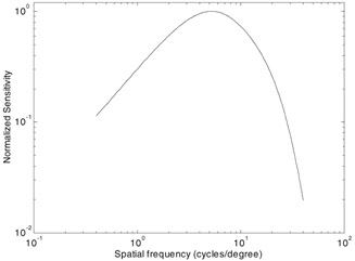
Figure 41.2: Normalized contrast sensitivity function.

Masking and Facilitation

Masking and facilitation are important aspects of the HVS in modelling the interactions between different image components present at the same spatial location. Masking/facilitation refers to the fact that the presence of one image component (called the mask) will decrease/increase the visibility of another image component (called the test signal). The mask generally reduces the visibility of the test signal in comparison with the case that the mask is absent. However, the mask may sometimes facilitate detection as well. Usually, the masking effect is the strongest when the mask and the test signal have similar frequency content and orientations. Most quality assessment methods incorporate one model of masking or the other, while some incorporate facilitation as well [1,18,25].

Pooling

Pooling refers to the task of arriving at a single measurement of quality, or a decision regarding the visibility of the artifacts, from the outputs of the visual streams. It is not quite understood as to how the HVS performs pooling. It is quite obvious that pooling involves cognition, where a perceptible distortion may be more annoying in some areas of the scene (such as human faces) than at others. However, most quality assessment metrics use Minkowski pooling to pool the error signal from the different frequency and orientation selective streams, as well as across spatial coordinates, to arrive at a fidelity measurement.

2.1.3 Summary

Summarizing the above discussion, an elaborate quality assessment algorithm may implement the following HVS features:

1. Eye optics modelled by a low-pass PSF.

2. Color processing.

3. Non-uniform retinal sampling.

4. Light adaptation (luminance masking).

5. Contrast sensitivity functions.

6. Spatial frequency, temporal frequency and orientation selective signal analysis.

7. Masking and facilitation.

8. Contrast response saturation.

9. Pooling.

2.2 General Framework of Error Sensitivity Based Metrics

Most HVS based quality assessment metrics share an error-sensitivity based paradigm, which aims to quantify the strength of the errors between the reference and the distorted signals in a perceptually meaningful way. Figure 41.3 shows a generic error-sensitivity based quality assessment framework that is based on HVS modelling. Most quality assessment algorithms that model the HVS can be explained with this framework, although they may differ in the specifics.

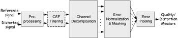
Figure 41.3: Framework of error sensitivity based quality assessment system. Note— the CSF feature can be implemented either as "CSF Filtering" or within "Error Normalization."

Pre-processing

The pre-processing stage may perform the following operations: alignment, transformations of color spaces, calibration for display devices, PSF filtering and light adaptation. First, the distorted and the reference signals need to be properly aligned. The distorted signal may be misaligned with respect to the reference, globally or locally, for various reasons during compression, processing, and transmission. Point-to-point correspondence between the reference and the distorted signals needs to be established. Second, it is sometimes preferable to transform the signal into a color space that conforms better to the HVS. Third, quality assessment metrics may need to convert the digital pixel values stored in the computer memory into luminance values of pixels on the display device through point-wise non-linear transformations. Fourth, a low-pass filter simulating the PSF of the eye optics may be applied. Finally, the reference and the distorted videos need to be converted into corresponding contrast stimuli to simulate light adaptation. There is no universally accepted definition of contrast for natural scenes. Many models work with band-limited contrast for complex natural scenes [26], which is tied with the channel decomposition. In this case, the contrast calculation is implemented later in the system, during or after the channel decomposition process.

CSF Filtering

CSF may be implemented before the channel decomposition using linear filters that approximate the frequency responses of the CSF. However, some metrics choose to implement CSF as weighting factors for channels after the channel decomposition.

Channel Decomposition

Quality metrics commonly model the frequency selective channels in the HVS within the constraints of application and computation. The channels serve to separate the visual stimulus into different spatial and temporal subbands. While some quality assessment algorithms implement sophisticated channel decompositions, simpler transforms such as the wavelet transform, or even the Discrete Cosine Transform (DCT) have been reported in the literature primarily due to their suitability for certain applications, rather than their accuracy in modelling the cortical neurons.

While the cortical receptive fields are well represented by 2D Gabor functions, the Gabor decomposition is difficult to compute and lacks some of the mathematical conveniences that are desired for good implementation, such as invertibility, reconstruction by addition, etc. Watson constructed the cortex transform [27] to model the frequency and orientation selective channels, which have similar profiles as 2D Gabor functions but are more convenient to implement. Channel decomposition models used by Watson, Daly [28,29], Lubin [17,18] and Teo and Heeger [1,25,30] attempt to model the HVS as closely as possible without incurring prohibitive implementation difficulties. The subband configurations for some of the models described in this chapter are given in Figure 41.4. Channels tuned to various temporal frequencies have also been reported in the literature [5,22,31,32].

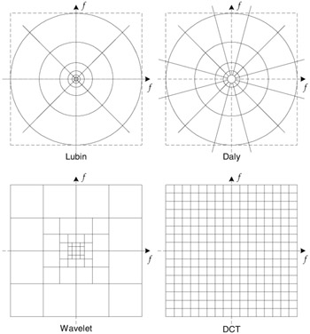
Figure 41.4: Frequency decompositions of various models.

Error Normalization and Masking

Error normalization and masking is typically implemented within each channel. Most models implement masking in the form of a gain-control mechanism that weights the error signal in a channel by a space-varying visibility threshold for that channel [33]. The visibility threshold adjustment at a point is calculated based on the energy of the reference signal (or both the reference and the distorted signals) in the neighbourhood of that point, as well as the HVS sensitivity for that channel in the absence of masking effects (also known as the base-sensitivity). Figure 41.5(a) shows how masking is typically implemented in a channel. For every channel the base error threshold (the minimum visible contrast of the error) is elevated to account for the presence of the masking signal. The threshold elevation is related to the contrast of the reference (or the distorted) signal in that channel through a relationship that is depicted in Figure 41.5(b). The elevated visibility threshold is then used to normalize the error signal. This normalization typically converts the error into units of Just Noticeable Difference (JND), where a JND of 1.0 denotes that the distortion at that point in that channel is just at the threshold of visibility. Some methods implement masking and facilitation as a manifestation of contrast response saturation. Figure 41.6 shows a set of curves each of which may represent the saturation characteristics of neurons in the HVS. Metrics may model masking with one or more of these curves.

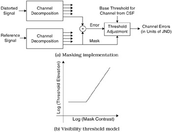
Figure 41.5: (a) Implementation of masking effect for channel based HVS models. (b) Visibility threshold model (simplified)— threshold elevation versus mask contrast.

Error Pooling

Error pooling is the process of combining the error signals in different channels into a single distortion/quality interpretation. For most quality assessment methods, pooling takes the form:

(41.3)

where e_l,k is the normalized and masked error of the k-th coefficient in the l-th channel, and β is a constant typically with a value between 1 and 4. This form of error pooling is commonly called Minkowski error pooling. Minkowski pooling may be performed over space (index k) and then over frequency (index l), or vice versa, with some non-linearity between them, or possibly with different exponents β. A spatial map indicating the relative importance of different regions may also be used to provide spatially variant weighting to different e_l,k [31, 34, 35].

2.3 Image Quality Assessment Algorithms

Most of the efforts in the research community have been focussed on the problem of image quality assessment, and only recently has video quality assessment received more attention. Current video quality assessment metrics use HVS models similar to those used in many image quality assessment metrics, with appropriate extensions to incorporate the temporal aspects of the HVS. In this section, we present some image quality assessment metrics that are based on the HVS error sensitivity paradigm. Later we will present some video quality assessment metrics. A more detailed review of image quality assessment metrics may be found in [2,36].

The visible differences predictor (VDP) by Daly [28,29] aims to compute a probability-of-detection map between the reference and the distorted signal. The value at each point in the map is the probability that a human observer will perceive a difference between the reference and the distorted images at that point. The reference and the distorted images (expressed in luminance values instead of pixels) are passed through a series of processes: point non-linearlity, CSF filtering, channel decomposition, contrast calculation, masking effect modelling, and probability-of-detection calculation. A modified cortex transform [27] is used for channel decomposition, which transforms the image signal into five spatial levels followed by six orientation levels, leading to a total of 31 independent channels (including the baseband). For each channel, a threshold elevation map is computed from the contrast in that channel. A psychometric function is used to convert error strengths (weighted by the threshold elevations) into a probability-of-detection map for each channel. Pooling is then carried out across the channels to obtain an overall detection map.

Lubin's algorithm [17, 18] also attempts to estimate a detection probability of the differences between the original and the distorted versions. A blur is applied to model the PSF of the eye optics. The signals are then re-sampled to reflect the photoreceptor sampling in the retina. A Laplacian pyramid [37] is used to decompose the images into seven resolutions (each resolution is one-half of the immediately higher one), followed by band-limited contrast calculations [26]. A set of orientation filters implemented through steerable filters of Freeman and Adelson [38] is then applied for orientation selectivity in four orientations. The CSF is modelled by normalizing the output of each frequency-selective channel by the base-sensitivity for that channel. Masking is implemented through a sigmoid non-linearity, after which the errors are convolved with disk-shaped kernels at each level before being pooled into a distortion map using Minkowski pooling across frequency. An additional pooling stage may be applied to obtain a single number for the entire image.

Teo and Heeger's metric [1,25,30] uses PSF modelling, luminance masking, channel decomposition, and contrast normalization. The channel decomposition process uses quadrature steerable filters [39] with six orientation levels and four spatial resolutions. A detection mechanism is implemented based on squared error. Masking is modelled through contrast normalization and response saturation. The contrast normalization is different from Daly's or Lubin's method in that they take the outputs of channels at all orientations at a particular resolution to perform the normalization. Thus, this model does not assume that the channels at the same resolution are independent. Only channels at different resolutions are considered to be independent. The output of the channel decomposition after contrast normalization is decomposed four-fold by passing through four non-linearities of shapes as illustrated in Figure 41.6, the parameters for which are optimized to fit the data from psychovisual experiments.

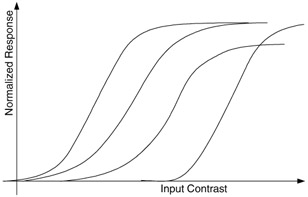
Figure 41.6: Non-linear contrast response saturation effects.

Watson's DCT metric [40] is based on an 8x8 DCT transform commonly used in image and video compression. Unlike the models above, this method partitions the spectrum into 64 uniform subbands (8 in each Cartesian dimension). After the block-based DCT and the associated subband contrasts are computed, a visibility threshold is calculated for each subband coefficient within each block using the base-sensitivity for that subband. The base sensitivities are derived empirically. The thresholds are corrected for luminance and texture masking. The error in each subband is weighted by the corresponding visibility threshold and pooled using Minkowski pooling spatially. Pooling across subbands is then performed using the Minkowski formulation with a different exponent.

Safranek-Johnston's perceptual image coder [41] incorporates a quality metric using a similar strategy as in Watson's DCT metric. The channel decomposition uses a generalized quadrature mirror filter (GQMF) [42] for analysis and synthesis. This transform splits the spectrum into 16 uniform subbands (four in each Cartesian dimension). Masking and pooling methods are similar to those in Watson's DCT metric.

Bradley [43] reports a wavelet visible difference predictor (WVDP), which is a simplification of Daly's VDP described above. He uses Watson's derivation of 9/7 Wavelet quantization-noise detection thresholds [44] for a 9/7 biorthogonal wavelet [45] and combines it with a threshold elevation and psychometric detection probability scheme similar to Daly's. Another wavelet based metric has been proposed by Lai and Kuo [6]. Their metric is based on the Haar Wavelet and their masking model can account for channel interactions as well as suprathreshold effects.

The quality metrics proposed above are scalar valued metrics. Damera-Venkata et al. proposed a metric for quantifying performance of image restoration systems, in which the degradation is modelled as a linear frequency distortion and additive noise injection [46]. Two complementary metrics were developed to separately quantify these distortions. They observed that if the additive noise is uncorrelated with the reference image, then an error measure from an HVS based metric will correlate well with the subjective judgement. Using a spatially adaptive restoration algorithm [47] (which was originally designed for inverse-halftoning), they isolate the effects of noise and linear frequency distortion. The noise is quantified using a multichannel HVS based metric. A distortion measure quantifies the spectral distortion between the reference and the model restored image.

Some researchers have attempted to measure image quality using single-channel models with the masking-effect models specifically targeting certain types of distortions, such as the blocking artifact. Blocking is recognized as one of the most annoying artifacts in block-DCT based image/video compression such as JPEG, especially at high compression ratios. In [48] and [49], Karunasekera and Kingsbury proposed a quality metric for blocking artifacts. Edge detection is performed first on the error image. An activity map is calculated from the reference image in the neighbourhood of the edges, and an activity-masked edge image is computed such that edges that occur in high activity areas are de-emphasized. The activity-masked edge image is adjusted for luminance masking. A non-linear transformation is applied before pooling. The parameters for the model are obtained from experiments that measure the sensitivity of human observers to edge artifacts embedded in narrow-band test patterns.

In [50], Chou and Li defined a peak signal to perceptible noise ratio (PSPNR), which is a single-channel metric. They model luminance masking and activity masking to obtain a JND profile. The PSPNR has the same definition as given in (2) except that the MSE expression is adjusted for the JND profile.

Another single-channel metric is the objective picture quality scale (PQS) by Miyahara [51]; a number of features that can capture various distortions are combined into one score. The method has also been extended for video quality assessment [52].

2.4 Video Quality Assessment Algorithms

One obvious way to implement video quality metrics is to apply a still image quality assessment metric on a frame-by-frame basis. However, a more sophisticated approach would model the temporal aspects of the HVS in the design of the metric. A number of algorithms have been proposed to extend the HVS features into the dimensions of time and motion [5,22,24,32,52–54]. A survey of video coding distortions can be found in [55]. A review of HVS modelling for video quality metrics is presented in [56].

In [53], Tan et al. implemented a Video Distortion Meter by using an image quality assessment metric followed by a "cognitive emulator" that models temporal effects such as smoothing and temporal masking of the frame quality measure, saturation and asymmetric tracking. Asymmetric tracking models the phenomenon that humans tend to notice a quality transition from good to poor more readily than a quality transition from poor to good.

Van den Branden Lambrecht et al. has extended the HVS modelling into the time dimension by modelling the temporal dimension of the CSF, and by generating two visual streams tuned to different temporal aspects of the stimulus from the output of each spatial channel [21,22,31,32]. The two streams model the transient and the sustained temporal mechanisms in the HVS. His proposed moving picture quality metric (MPQM) consists of a channel decomposition into four scales, four orientations and two temporal streams. The resulting channel outputs are subtracted to create the error signal. Masking is implemented by normalization of the channel errors by the stimulus dependent visibility thresholds (similar to those used in still image quality assessment metrics). Motion rendering quality assessment has also been proposed by extending the MPQM by extraction of motion information [32].

In [5], Winkler presented a quality assessment metric for color video. The algorithm uses a color space transformation and applies the quality assessment metric on each transformed color channel. Two temporal streams are generated using IIR filters, with spatial decomposition into five subband levels and four orientations. Channels are weighted by the corresponding CSF, and masking is implemented based on the excitatory-inhibitory masking model proposed by Watson and Solomon [33].

Watson's digital video quality (DVQ) metric operates in the DCT domain and is therefore more attractive from an implementation point of view [24,57] since the DCT is efficient to implement and most video coding standards are based on the DCT. A three-dimensional visibility threshold model for spatiotemporal DCT channels was proposed. The DVQ algorithm first takes the DCT of the reference and the distorted signals, respectively. It then computes local contrast, applies temporal CSF filtering, and converts the results into JND units by normalizing them with the visibility thresholds, following which the error signal is computed. Finally, masking and pooling are applied to the error signal. DVQ implements color transformation before applying the metric to each of the chrominance dimensions.

Another metric that models the temporal aspects of HVS is presented by Tan and Ghanbari [54], which aims to evaluate the quality of MPEG video and combines a typical error-sensitivity based perceptual model with a blockiness measurement model. The perceptual model consists of display gamma correction, point non-linearity, contrast calculation, spatial CSF filtering, temporal filtering, frequency decomposition into two channels (diagonal and horizontal/vertical), contrast response non-linearity, error averaging, masking, pooling, temporal averaging and motion masking. The blockiness detector is based on harmonic analysis of the block-edge signal, combined with a visual masking model. The final quality score is either the perceptual model score or the blockiness detector score, based on the amount of blockiness artifact detected.

In [58], Yu et al. propose a video quality metric based on the extension of the perceptual distortion metric by Winkler [5] to a perceptual blocking distortion metric. The parameters for the models are obtained by minimizing the error in quality predictions for video sequences obtained from VQEG subjective testing database. This is in contrast to most methods that obtain parameters to fit threshold psychovisual experiments with simple patterns. They specifically address the blocking artifact by pooling spatially over those areas where blocking effects are dominant.

There are several implementation issues that need to be considered before developing a practical video quality assessment system. One important factor affecting the feasibility of a quality metric for video is its computational complexity. While complex quality assessment methods may model the HVS more accurately, their computational complexity may be prohibitively large for many platforms, especially for real-time quality assessment of high-resolution video. Memory requirements are another important issue. For example, in order to implement temporal filtering, a large memory space may be needed to store a number of video frames, which is expensive on many platforms. Another problem of HVS based metrics might be their dependence on viewing configurations, which include the resolution of the display devices, the nonlinear relationships between the digital pixel values and the output luminance values, and the viewing distance of the observers. Most models either require that viewing configurations be known or simply assume a fixed set of configurations. How these metrics would perform when the configurations are unknown or the assumptions about the configurations do not hold is another issue that needs to be studied.

2.5 Limitations

The underlying principle of visual error sensitivity based algorithms is to predict perceptual quality by quantifying perceptible errors. This is accomplished by simulating the perceptual quality related functional components of the HVS. However, the HVS is an extremely complicated, highly non-linear system, and the current understanding of the HVS is limited. How far the error sensitivity based framework can reach is a question that may need many years to answer.

It is worth noting that most error sensitivity based approaches, explicitly or implicitly, make a number of assumptions. The following is an incomplete list (Note: a specific model may use a subset of these assumptions):

1. The reference signal is of perfect quality.

2. Light adaptation follows the Weber's law.

3. After light adaptation, the optics of the eye can be modelled as a linear time-invariant system characterized by a PSF.

4. There exist frequency, orientation and temporal selectivity visual channels in the HVS, and the channel responses can be modelled by a discrete set of linear decompositions.

5. Although the contrast definitions of simple patterns used in psychovisual experiments and the contrast definitions of complex natural images may be different, they are consistent with each other.

6. The relative visual error sensitivity between different spatial and/or temporal frequency channels can be normalized using a bandpass or lowpass CSF.

7. The channel decomposition is lossless or nearly lossless in terms of visual importance, in the sense that the transformed signals maintain most of the information needed to assess the image quality.

8. The channel decomposition effectively decorrelates the image structure, such that the inter- and intra-channel interactions between transformed coefficients can be modelled using a masking model, in which the strength of the mask is determined by the magnitudes (not structures) of the coefficients. After masking, the perceived error of each coefficient can be evaluated individually.

9. For a single coefficient in each channel, after error normalization and masking, the relationship between the magnitude of the error, e_l,k, and the distortion perceived by the HVS, d_l,k , can be modelled as a nonlinear function: .

10. The overall perceived distortion monotonically increases with the summation of the perceived errors of all coefficients in all channels.

11. The overall framework covers a complete set of dominant factors (light adaptation, PSF of the eye optics, CSF of the frequency responses, masking effects, etc.) that affect the perceptual quality of the observed image.

12. Higher level processes happening in the human brain, such as pattern matching with memory and cognitive understanding, are less important for predicting perceptual image quality.

13. Active visual processes, such as the change of fixation points and the adaptive adjustment of spatial resolution because of attention, are less important for predicting perceptual image quality.

Depending on the application environment, some of the above assumptions are valid or practically reasonable. For example, in image and video compression and communication applications, assuming a perfect original image or video signal (Assumption 1) is acceptable. However, from a more general point of view, many of the assumptions are arguable and need to be validated. We believe that there are several problems that are critical for justifying the usefulness of the general error-sensitivity based framework.

The Suprathreshold Problem

Most psychophysical subjective experiments are conducted near the threshold of visibility, typically using a 2-Alternative Forced-Choice (2AFC) method [14,59].

The 2AFC method is used to determine the values of stimuli strength (also called the threshold strength) at which the stimuli are just visible. These measured threshold values are then used to define visual error sensitivity models, such as the CSF and the various masking effect models. However, there is not sufficient evidence available from vision research to support the presumption that these measurement results can be generalized to quantify distortions much larger than just visible, which is the case for a majority of image processing applications. This may lead to several problems with respect to the framework. One problem is that when the error in a visual channel is larger than the threshold of visibility, it is hard to design experiments to validate Assumption 9. Another problem is regarding Assumption 6, which uses the just noticeable visual error threshold to normalize the errors between different frequency channels. The question is: when the errors are much larger than the thresholds, can the relative errors between different channels be normalized using the visibility thresholds?

The Natural Image Complexity Problem

Most psychovisual experimental results published in the literature are conducted using relatively simple patterns, such as sinusoidal gratings, Gabor patches, simple geometrical shapes, transform basis functions, or random noise patterns. The CSF is obtained from threshold experiments using single frequency patterns. The masking experiments usually involve two (or a few) different patterns. However, all such patterns are much simpler than real world images, which can usually be thought of as a superposition of a large number of different simple patterns. Are these simple-pattern experiments sufficient for us to build a model that can predict the quality of complex natural images? Can we generalize the model for the interactions between a few simple patterns to model the interactions between tens or hundreds of patterns?

The Minkowski Error Pooling Problem

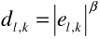
The widely used Minkowski error summation formula (3) is based on signal differencing between two signals, which may not capture the structural changes between the two signals. An example is given in Figure 41.7, where two test signals, test signals 1 (up-left) and 2 (up-right), are generated from the original signal (up-center). Test signal 1 is obtained by adding a constant number to each sample point, while the signs of the constant number added to test signal 2 are randomly chosen to be positive or negative. The structural information of the original signal is almost completely lost in test signal 2, but preserved very well in test signal 1. In order to calculate the Minkowski error metric, we first subtract the original signal from the test signals, leading to the error signals 1 and 2, which have very different structures. However, applying the absolute operator on the error signals results in exactly the same absolute error signals. The final Minkowski error measures of the two test signals are equal, no matter how the β value is selected. This example not only demonstrates that "structure-preservation" ability is an important factor in measuring the similarity between signals, but also shows that Minkowski error pooling is inefficient in capturing the structures of errors and is a "structural information lossy" metric. Obviously, in this specific example, the problem may be solved by applying a spatial frequency channel decomposition on the error signals and weighting the errors differently in different channels with a CSF. However, the decomposed signals may still exhibit different structures in different channels (for example, assume that the test signals in Figure 41.7 are from certain channels instead of the spatial domain), then the "structural information lossy" weakness of the Minkowski metric may still play a role, unless the decomposition process strongly decorrelates the image structure, as described by Assumption 8, such that the correlation between adjacent samples of the decomposed signal is very small (in that case, the decomposed signal in a channel would look like random noise). However, this is apparently not the case for a linear channel decomposition method such as the wavelet transform. It has been shown that a strong correlation or dependency exists between intra- and inter-channel wavelet coefficients of natural images [60,61]. In fact, without exploiting this strong dependency, state-of-the-art wavelet image compression techniques, such as embedded zerotree wavelet (EZW) coding [62], set partitioning in hierarchical trees (SPIHT) algorithm [63], and JPEG2000 [64] would not be successful.

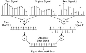
Figure 41.7: Illustration of Minkowski error pooling.

The Cognitive Interaction Problem

It is clear that cognitive understanding and active visual process (e.g., change of fixations) play roles in evaluating the quality of images. For example, a human observer will give different quality scores to the same image if s/he is instructed with different visual tasks [2,65]. Prior information regarding the image content, or attention and fixation, may also affect the evaluation of the image quality [2,66]. For example, it is shown in [67] that in a video conferencing environment, "the difference between sensitivity to foreground and background degradation is increased by the presence of audio corresponding to speech of the foreground person" [67]. Currently, most image and video quality metrics do not consider these effects. How these effects change the perceived image quality, how strong these effects compare with other HVS features employed in the current quality assessment models, and how to incorporate these effects into a quality assessment model have not yet been deeply investigated.