3. Experimental Results

3. Experimental Results

In this section, we present experimental results to demonstrate the performance of the ViSig method. All experiments use color histograms as video frame features described in more detail in Section 3.1. Two sets of experiments are performed. Results of a number of controlled simulations are presented in Section 3.2 to demonstrate the heuristics proposed in Section 2. In Section 3.3, we apply the ViSig method to a large set of real-life web video sequences.

3.1 Image Feature

In our experiments, we use four 178-bin color histograms on the Hue-Saturation-Value (HSV) color space to represent each individual frame in a video. Color histogram is one of the most commonly used image features in content-based retrieval system. The quantization of the color space used in the histogram is shown in Figure 28.4. This quantization is similar to the one used in [19]. The saturation (radial) dimension is uniformly quantized into 3.5 bins, with the half bin at the origin. The hue (angular) dimension is uniformly quantized at 20 -step size, resulting in 18 sectors. The quantization for the value dimension depends on the saturation value. For those colors with the saturation values near zero, a finer quantizer of 16 bins is used to better differentiate between gray-scale colors. For the rest of the color space, the value dimension is uniformly quantized into three bins. The histogram is normalized such that the sum of all the bins equals one. In order to incorporate spatial information into the image feature, the image is partitioned into four quadrants, with each quadrant having its own color histogram. As a result, the total dimension of a single feature vector becomes 712.

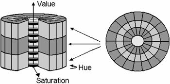
Figure 28.4: Quantization of the HSV color space.

We use two distance measurements in comparing color histograms: the l₁ metric and a modified version of the l₁ distance with dominant color first removed. The l₁ metric on color histogram was first used in [20] for image retrieval. It is defined by the sum of the absolute difference between each bin of the two histograms. We denote the l₁ metric between two feature vectors x and y as d(x, y), with its precise definition stated below:

(28.16)

where x_i and y_i for i ∈ {1,2,3,4} represent the quadrant color histograms from the two image feature vectors. A small d() value usually indicates visual similarity, except when two images share the same background color. In those cases, the metric d() does not correctly reflect the differences in the foreground as it is overwhelmed by the dominant background color. Such scenarios are quite common among the videos found on the web. Examples include those video sequences composed of presentation slides or graphical plots in scientific experiments. To mitigate this problem, we develop a new distance measurement which first removes the dominant color, then computes the l₁ metric for the rest of the color bins, and finally re-normalizes the result to the proper dynamic range. Specifically, this new distance measurement d'(x,y) between two feature vectors x and y can be defined as follows:

(28.17)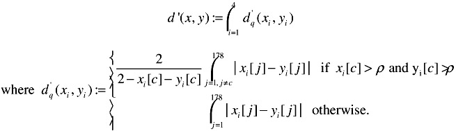

In Equation (28.17), the dominant color is defined to be the color c with bin value exceeding the Dominant Color Threshold ρ . ρ has to be larger than or equal to 0.5 to guarantee a single dominant color. We set ρ = 0.5 in our experiments. When the two feature vectors share no common dominant color, d'() reduces to d().

Notice that the modified l₁ distance d'() is not a metric. Specifically, it does not satisfy the triangle inequality. Thus, it cannot be directly applied to measuring video similarity. The l₁ metric d() is used in most of the experiments described in Sections 3.2 and 3.3. We only use d'() as a post-processing step to improve the retrieval performance in Section 3.3. The process is as follows: first, given a query video X, we declare a video Y in a large database to be similar to X if the VSS, either the Basic or Ranked version, between the corresponding ViSig and exceeds a certain threshold λ. The l₁ metric d() is first used in computing all the VSS's. Denote the set of all similar video sequences Y in the database as ret(X,ε). Due to the limitation of l₁ metric, it is possible that some of the video sequences in Π may share the same background as the query video but are visually very different. In the second step, we compute the d'() -based VSS between and all the ViSig's in ret(X,ε). Only those ViSig's whose VSS with larger than λ are retained in ret(X,ε), and returned to the user as the final retrieval results.

3.2 Simulation Experiments

In this section, we present experimental results to verify the heuristics proposed in Section 2. In the first experiment, we demonstrate the effect of the choice of SV's on approximating the IVS by the ViSig method. We perform the experiment on a set of 15 video sequences selected from the MPEG-7 video data set [21]. ^[4] This set includes a wide variety of video content including documentaries, cartoons, and television drama, etc. The average length of the test sequences is 30 minutes. We randomly drop frames from each sequence to artificially create similar versions at different levels of IVS. ViSig's with respect to two different sets of SV's are created for all the sequences and their similar versions. The first set of SV's are independent random vectors, uniformly distributed on the high-dimensional histogram space. To generate such random vectors, we follow the algorithm described in [22]. The second set of SV's are randomly selected from a set of images in the Corel Stock Photo Collection. These images represent a diverse set of real-life images, and thus provide a reasonably good approximation to the feature vector distribution of the test sequences. We randomly choose around 4000 images from the Corel collection, and generate the required SV's using the SV Generation Method, with ε_SV set to 2.0, as described in Section 2.4. Table 28.1 shows the VSS_b with m = 100 SV's per ViSig at IVS levels of 0.8, 0.6, 0.4 and 0.2. VSS_b based on Corel images are closer to the underlying IVS than those based on random vectors. In addition, the fluctuations in the estimates, as indicated by the standard deviations, are far smaller with the Corel images. The experiment thus shows that it is advantageous to use SV's that approximate the feature vector distribution of the target data.

Table 28.1: Comparison between using uniform random and Corel image SV's. The second through fifth columns are the results of using uniform random SV's and the rest are the Corel image SV's. Each row contains the results of a specific test video at IVS levels 0.8, 0.6, 0.4 and 0.2. The last two rows are the averages and standard deviations over all the test sequences.

Seed Vectors	Uniform Random				Corel Images
IVS	0.8	0.6	0.4	0.2	0.8	0.6	0.4	0.2
v1_1	0.59	0.37	0.49	0.20	0.85	0.50	0.49	0.23
v1_2	0.56	0.38	0.31	0.05	0.82	0.63	0.41	0.18
v3	0.96	0.09	0.06	0.02	0.82	0.52	0.40	0.21
v4	0.82	0.75	0.55	0.24	0.92	0.44	0.48	0.25
v5_1	0.99	0.71	0.28	0.18	0.76	0.66	0.39	0.12
v5_2	0.84	0.35	0.17	0.29	0.81	0.68	0.36	0.10
v5_3	0.97	0.36	0.74	0.07	0.76	0.59	0.51	0.15
v6	1.00	0.00	0.00	0.00	0.79	0.61	0.46	0.25
v7	0.95	0.89	0.95	0.60	0.86	0.60	0.49	0.16
v8_1	0.72	0.70	0.47	0.17	0.88	0.69	0.38	0.20
v8_2	1.00	0.15	0.91	0.01	0.86	0.53	0.35	0.21
v9_1	0.95	0.85	0.54	0.15	0.93	0.56	0.44	0.18
v9_2	0.85	0.70	0.67	0.41	0.86	0.56	0.39	0.17
v9_3	0.90	0.51	0.30	0.10	0.78	0.70	0.45	0.15
v9_4	1.00	0.67	0.00	0.00	0.72	0.45	0.42	0.24
Average	0.873	0.499	0.429	0.166	0.828	0.581	0.428	0.187
Stddev	0.146	0.281	0.306	0.169	0.060	0.083	0.051	0.046

In the second experiment, we compare the Basic ViSig method with the Ranked ViSig method in identifying sequences with IVS one under the presence of small feature vector displacements. As described in Section 2.5, when two frames from two video sequences are separated by a small ε, the Basic ViSig method may underestimate the IVS because of the presence of VG. To combat such a problem, we propose the Ranked ViSig method in Section 2.5. In this experiment, we create similar video by adding noise to individual frames. Most of the real-life noise processes such as compression are highly video dependent, and cannot provide a wide-range of controlled noise levels for our experiment. As such, we introduce artificial noise that directly corresponds to the different noise levels as measured by our frame metric. As shown in [20], the l₁ metric used in histograms is equal to twice the percentage of the pixels between two images that are of different colors. For example, if the l₁ metric between two histograms is 0.4, it implies that 20% of the pixels in the images have different color. Thus, to inject a particular ε noise level to a frame, we determine the fraction of the pixels that need to have different colors and randomly assign colors to them. The color assignment is performed in such a way that ε noise level is achieved exactly. Five ε levels are tested in our experiments: 0.2, 0.4, 0.8, 1.2 and 1.6. In our definition of a feature vector, four histograms are used per frame. This means that an ε of, for example, 1.6 results in an average noise level of 0.4 for each histogram. After injecting noise to create the similar video, a 100-frame Basic ViSig (m = 100) and a 500-frame Ranked ViSig (m' = 500) are generated for each video. All SV's are randomly sampled from the Corel dataset. To ensure the same computational complexity between the two methods, the top m/2 = 50 Ranked ViSig frames are used in computing VSS_r. The results are shown in Table 28.2. The averages and standard deviations over the entire set are shown in the last two rows. Since the IVS is fixed at one, the closer the measured similarity is to one, the better the approximation is. Even though both methods show a general trend of increasing error as the noise level increase, as expected, VSS_r measurements are much closer to one than VSS_b.

Table 28.2: Comparison between VSS_b and VSS_r under different level of perturbation. The table follows the same format as in Table 28.1. The perturbation levels ε tested are 0.2, 0.4. 0.8, 1.2 and 1.6.

Algo.	VSSb					VSSr
ε	0.2	0.4	0.8	1.2	1.6	0.2	0.4	0.8	1.2	1.6
v1_1	0.89	0.76	0.62	0.54	0.36	1.00	1.00	0.90	0.87	0.74
v1_2	0.81	0.73	0.55	0.47	0.34	1.00	0.98	0.83	0.73	0.62
v3	0.90	0.76	0.70	0.42	0.36	1.00	1.00	0.96	0.87	0.72
v4	0.86	0.74	0.64	0.48	0.38	1.00	1.00	0.96	0.83	0.74
v5_1	0.90	0.77	0.64	0.45	0.41	1.00	1.00	0.98	0.79	0.86
v5_2	0.96	0.81	0.52	0.66	0.56	1.00	1.00	1.00	0.86	0.78
v5_3	0.88	0.83	0.59	0.42	0.39	1.00	1.00	0.90	0.83	0.74
v6	0.88	0.72	0.64	0.49	0.49	1.00	1.00	0.98	0.92	0.78
v7	0.89	0.84	0.68	0.46	0.43	1.00	1.00	1.00	0.91	0.78
v8_1	0.85	0.67	0.58	0.52	0.30	1.00	1.00	0.87	0.79	0.73
v8_2	0.90	0.80	0.72	0.59	0.56	1.00	1.00	0.99	0.95	0.86
v9_1	0.87	0.77	0.62	0.67	0.48	1.00	0.99	0.89	0.84	0.82
v9_2	0.82	0.70	0.55	0.50	0.37	1.00	1.00	0.90	0.78	0.59
v9_3	0.86	0.65	0.66	0.49	0.40	1.00	1.00	0.91	0.70	0.58
v9_4	0.92	0.86	0.71	0.61	0.53	1.00	1.00	0.93	0.89	0.82
Avg.	0.879	0.761	0.628	0.518	0.424	1.000	0.998	0.933	0.837	0.744
Stdev	0.038	0.061	0.061	0.080	0.082	0.000	0.006	0.052	0.070	0.088

3.3 Web Video Experiments

To further demonstrate how the ViSig method can be applied to a realistic application, we test our algorithms on a large dataset of web video and measure their retrieval performance using a ground-truth set. Its retrieval performance is further compared with another summarization technique called the k-medoid. k-medoid was first proposed in [14] as a clustering method used in general metric spaces. One version of k-medoid was used by Chang et al. for extracting a predefined number of representative frames from a video [7]. Given a l -frame video X = {x_t :t =1,2,...,l}, the k-medoid of X is defined to be a set of k frames in X that minimize the following cost function:

(28.18)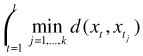

Due to the large number of possible choices in selecting k frames from a set, it is computationally impractical to precisely solve this minimization problem. In our experiments, we use the PAM algorithm proposed in [14] to compute an approximation to the k-medoid. This is an iterative algorithm and the time complexity for each iteration is on the order of l². After computing the k-medoid for each video, we declare two video sequences to be similar if the minimum distance between frames in their corresponding k-medoids is less than or equal to ε.

The dataset for the experiments is a collection of 46,356 video sequences, crawled from the web between August and December, 1999. The URL addresses of these video sequences are obtained by sending dictionary entries as text queries to the AltaVista video search engine [23]. Details about our data collection process can be found in [24]. The statistics of the four most abundant formats of video collected are shown in Table 28.3.

Table 28.3: Statistics of collected web video sequences

Video Type	% over all clips	Duration ( stddev) minutes
MPEG	31	0.36 0.7
QuickTime	30	0.51 0.6
RealVideo	22	9.57 18.5
AVI	16	0.16 0.3

The ground-truth is a set of manually identified clusters of almost-identical video sequences. We adopt a best-effort approach to obtain such a ground-truth. This approach is similar to the pooling method [25] commonly used in text retrieval systems. The basic idea of pooling is to send the same queries to different automatic retrieval systems, whose top-ranked results are pooled together and examined by human experts to identify the truly relevant ones. For our system, the first step is to use meta-data terms to identify the initial ground-truth clusters. Meta-data terms are extracted from the URL addresses and other auxiliary information for each video in the dataset [26]. All video sequences containing at least one of the top 1000 most frequently used meta-data terms are manually examined and grouped into clusters of similar video. Clusters which are significantly larger than others are removed to prevent bias. We obtain 107 clusters which form the initial ground-truth clusters. This method, however, may not be able to identify all the video clips in the dataset that are similar to those already in the ground-truth clusters. We further examine those video sequences in the dataset that share at least one meta-data term with the ground-truth video, and add any similar video to the corresponding clusters. In addition to meta-data, k-medoid is also used as an alternative visual similarity scheme to enlarge the ground-truth. A 7-frame k-medoid is generated for each video. For each video X in the ground-truth, we identify 100 video sequences in the dataset that are closest to X in terms of the minimum distance between their k-medoids, and manually examine them to search for any sequence that is visually similar to X. As a result, we obtain a ground-truth set consisting of 443 video sequences in 107 clusters. The cluster size ranges from 2 to 20, with average size equal to 4.1. The ground-truth clusters serve as the subjective truth for comparison against those video sequences identified as similar by the ViSig method.

When using the ViSig method to identify similar video sequences, we declare two sequences to be similar if their VSS_b or VSS_r is larger than a certain threshold λ ∈ [0,1]. In the experiments, we fix λ at 0.5 and report the retrieval results for different numbers of ViSig frames, m, and the Frame Similarity Threshold, ε. Our choice of fixing λ at 0.5 can be rationalized as follows: as the dataset consists of extremely heterogeneous contents, it is rare to find partially similar video sequences. We notice that most video sequences in our dataset are either very similar to each other, or not similar at all. If ε is appropriately chosen to match subjective similarity, and m is large enough to keep sampling error small, we would expect the VSS for an arbitrary pair of ViSig's to be close to either one or zero, corresponding to either similar or dissimilar video sequences in the dataset. We thus fix λ at 0.5 to balance the possible false-positive and false-negative errors, and vary ε to trace the whole spectrum of retrieval performance. To accommodate such a testing strategy, we make a minor modification in the Ranked ViSig method: recall that we use the Ranking Function Q() as defined in Equation (28.14) to rank all frames in a ViSig. Since Q() depends on ε and its computation requires the entire video sequence, it is cumbersome to recompute it whenever a different ε is used. ε is used in the Q() function to identify the clustering structure within a single video. Since most video sequences are compactly clustered, we notice that their Q() values remain roughly constant for a large range of ε. As a result, we a priori fix ε to be 2.0 to compute Q(), and do not recompute them even when we modify ε to obtain different retrieval results.

The performance measurements used in our experiments are recall and precision as defined below. Let A be the web video dataset and Φ be the ground-truth set. For a video X ∈ Φ, we define the Relevant Set to X, rel(X), to be the ground-truth cluster that contains X, minus X itself. Also recall the definition of the Return Set to X, ret(X,ε), from Section 3.1, as the set of video sequences in the database which are declared to be similar to X by the ViSig method, i.e., ret(X,ε):={Y ∈ ∧: vss(,) ≤ λ}\{X}. vss can be either VSS_b or VSS_r. By comparing the Return and Relevant Sets of the entire ground-truth, we can define the Recall and Precision as follows:

Thus, recall computes the fraction of all ground-truth video sequences that can be retrieved by the algorithm. Precision measures the fraction retrieved by the algorithm that is relevant. By varying ε, we can measure the retrieval performance of the ViSig method for a wide range of recall values.

The goal of the first experiment is to compare the retrieval performance between the Basic and the Ranked ViSig methods at different ViSig sizes. The modified l₁ distance on the color histogram is used in this experiment. SV's are randomly selected by the SV Generation Method, with ε_sv set to 2.0, from a set of keyframes representing the video sequences in the dataset. These keyframes are extracted by the AltaVista search engine and captured during data collection process; each video is represented by a single keyframe. For the Ranked ViSig method, m' = 100 keyframes are randomly selected from the keyframe set to produce the SV set which is used for all ViSig sizes, m. For each ViSig size in the Basic ViSig method, we average the results of four independent sets of randomly selected keyframes in order to smooth out the statistical variation due to the limited ViSig sizes. The plots in Figure 28.5(a) show the precision versus recall curves for four different ViSig sizes: m = 2, 6, 10 and 14. The Ranked ViSig method outperforms the Basic ViSig method in all four cases. Figure 28.5(b) shows the Ranked method's results across different ViSig sizes. There is a substantial gain in performance when the ViSig size is increased from two to six. Further increase in ViSig size does not produce much significant gain. The precision-recall curves all decline sharply once they reach beyond 75% for recall and 90% for precision. Thus, six frames per ViSig is adequate in retrieving ground-truth from the dataset.

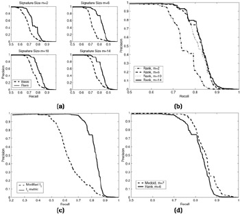
Figure 28.5: Precision-recall plots for web video experiments— (a) Comparisons between the Basic (broken-line) and Ranked (solid) ViSig methods for four different ViSig sizes— m=2, 6, 10, 14; (b) Ranked ViSig methods for the same set of ViSig sizes; (c) Ranked ViSig methods with m=6 based on l₁, metric (broken) and modified l₁ distance (solid) on color histograms; (d) Comparison between the Ranked ViSig method with m=6 (solid) and k-medoid with 7 representative frames (broken).

In the second experiment, we test the difference between using the modified l₁ distance and the l₂ metric on the color histogram. The same Ranked ViSig method with six ViSig frames is used. Figure 28.5(c) shows that the modified l₁ distance significantly outperforms the straightforward l₁ metric. Finally, we compare the retrieval performance between k-medoid and the Ranked ViSig method. Each video in the database is represented by seven medoids generated by the PAM algorithm. We plot the precision-recall curves for k-medoid and the six-frame Ranked ViSig method in Figure 28.5(d). The k-medoid technique provides a slightly better retrieval performance. The advantages seem to be small considering the complexity advantage of the ViSig method over the PAM algorithm. First, computing VSS_r needs six metric computations but comparing two 7-medoid representations requires 49. Second, the ViSig method generates ViSig's in O(l) time with l being the number of frames in a video, while the PAM algorithm is an iterative O(l²) algorithm.

^[4]The test set includes video sequences from MPEG-7 video CD's v1, v3, v4, v5, v6, v7, v8 and v9. We denote each test sequence by the CD they are in, followed by a number such as v8_1 if there are multiple sequences in the same CD.