4. A Hierarchical Fusion Model

4. A Hierarchical Fusion Model

In this paper, we discuss the problem of fusing multiple feature streams enjoying spatio-temporal support in different modalities. We present a hierarchical fusion model (see Figure 2.8), which makes use of late integration of intermediate decisions.

To solve the problem we propose a Hierarchical duration dependent input output Markov model. There are four main considerations that have led us to the particular choice of the fusion architecture.

• We argue that the different streams contain information which is correlated to one another only at a high level. This assumption allows us to process output of each source independently of one another. Since these sources may contain information which has highly temporal structure, we propose the use of hidden Markov models. These models are learned from the data and then we decode the hidden state sequence, characterizing the information describing the source at any given time. This assumption leads us to a hierarchical approach.

• We argue that the different sources contain independent information. At high level, the output of one source is essentially independent of the information contained in the other. However, conditioned upon a particular bi-modal concept, these different sources may be dependent on one another. This suggests the use of an alternative dependence assumption contrary to conventional causal models like HMMs. This is illustrated in Figures 2.3 and 2.4.

  
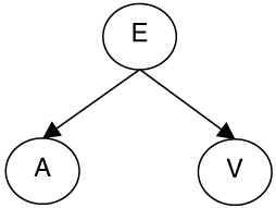
  Figure 2.3: Consider the multimodal concept represented by node E and multimodal features represented by nodes A and V in this Bayesian network. The network implies that features A and V are independent given concept E.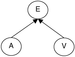

  
  Figure 2.4: Consider the multimodal concept represented by node E and multimodal features represented by nodes A and V in this Bayesian network. The network implies that features A and V are dependent given concept E.

  Note the difference between the assumptions implied by Figures 2.3 and 2.4. This idea can be explained with an example event, say an explosion. Suppose the node E represents event explosion and the nodes A and V represent some high characterization of audio and visual features. According to Figure 2.3 given the fact that an explosion is taking place, the audio and visual representations are independent. This means that once we know an explosion event is taking place, there is no information in either channel for the other. On the contrary Figure 2.4 implies that given an explosion event the audiovisual representations are dependent. This means that the audio channel and video channel convey information about each other only if the presence of event explosion is known. These are two very different views to the problem of modeling dependence between multiple modalities.

• We want to model temporal events. We therefore need to expand the model in Figure 2.4 to handle temporal dependecy in the event E. We make the usual Markovian assumption thus making the variable E at any time dependent only on its value at the previous time instant. This leads to an input output Markov model (IOMM). This is shown in Figure 2.5.

  
  Figure 2.5: This figure illustrates the Markovian transition of the input output Markov model. Random variable E can be present in one of the two states. The model characterizes the transition probabilities and the dependence of these on input sequence y.

• Finally, an important characteristic of semantic concepts in videos is their duration. This points to the important limitation of hidden Markov models. In HMMs the probability of staying in any particular state decays exponentially. This is the direct outcome of the one Markov property of these models. To alleviate this problem, we explicitly model these probabilities. This leads us to what we call duration dependent input output Markov model. Note that because of this explicit modeling of the state duration, these are not really one Markov models but are what have been called in the past semi-Markov models. This leads to the duration dependent input output Markov model (DDIOMM) as shown in Figure 2.6.

  
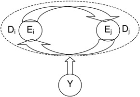
  Figure 2.6: This figure illustrates the Markovian transition of the input output Markov model along with duration models for stay in each state. Random variable E can be present in one of the two states. The model characterizes the transition probabilities and the dependence of these on input sequence y and duration of stay in any state. Note that missing self transition arrows.

Figure 2.7 shows the temporally rolled out Hierarchical model. This model takes as input, data from multiple sensors, which in the case of videos reduces to two streams Audio and Video. Figure 2.8 shows these two streams with one referring to audio features or observations AO₁,.,AO _T and the other to video features VO₁,.,VO _T. The media information represented by these features is modeled using hidden Markov models which here are referred to as media HMM as these are used to model each media. Each state in the media HMMs represents a stationary distribution and by using the Viterbi decoder over each feature stream, we essentially cluster features spatio-temporally and quantize them through state identities. State-sequence-based processing using trained HMMs can be thought of as a form of guided spatio-temporal vector quantization for reducing the dimensionality of the feature vectors from multiple streams [13].

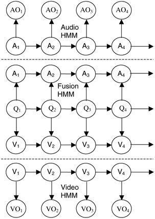
Figure 2.7: Hierarchical multimedia fusion using HMM. The media HMMs are responsible for mapping media observations to state sequences.

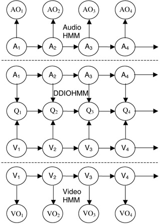
Figure 2.8: Hierarchical multimedia fusion. The media HMMs are responsible for mapping media observations to state sequences. The fusion model, which lies between the dotted lines, uses these state sequences as inputs and maps them to output decision sequences.

Once the individual streams have been modeled, inferencing is done to decode the state sequence for each stream of features. More formally, consider S streams of features. For each stream, consider feature vectors ,…, corresponding to time instants t=1,.,T . Consider two hypotheses H_i, i∈ {0,1} corresponding to the presence and absence of an event E in the feature stream. Under each hypothesis we assume that the feature stream is generated by a hidden Markov model [26] (the parameters of the HMM under each hypothesis are learned using the EM algorithm [26]). Maximum likelihood detection is used to detect the underlying hypothesis for a given sequence of features observed and then the corresponding hidden state sequence is obtained by using the Viterbi decoding (explained later). Once the state sequence for each feature stream is obtained, we can use these intermediate-level decisions from that feature stream [13] in a hierarchical approach.

Hierarchical models use these state sequences to do the inferencing. Figure 7 shows the fusion model, where standard HMM is used for fusing the different modalities. However this model has many limitations - it assumes the different streams are independent for a particular concept and models a exponentially decaying distribution for a particular event, which as discussed is not true in general.

Figure 2.8 illustrates in Hierarchical structure that uses DDIOMM. DDIOMM helps us to get around these, providing a more suitable fusion architecture. It is discussed in more detail in the next section.

4.1 The Duration Dependent Input Output Markov Model

Consider a sequence γ of symbols y₁,.,y T where y_i∈{1,.,N}. Consider another sequence Q of symbols q₁,.,q _T, where q_i∈{1,.,M}. The model between the dotted lines in Figure 2.8 illustrates a Bayesian network involving these two sequences. Here y={A,V} (i.e., Cartesian product of the audio and video sequence). This network can be thought of as a mapping of the input sequence γ to the output sequence Q. We term this network the Input Output Markov Model. This network is close in spirit to the input output hidden Markov model [47].

The transition in the output sequence is initially assumed to be Markovian. This leads to an exponential duration density model. Let us define A={A_ijk}, i,j∈{1,.,M}, k ∈{1,.,N} as the map. A_ijk=P(q_t=j|q_t-1=i,y_t=k) is estimated from the training data through frequency counting and tells us the probability of the current decision state given the current input symbol and the previous state. Once A is estimated, we can then predict the output sequence Q, given the input sequence γ using Viterbi decoding.

The algorithm for decoding the decision is presented below.

(2.5)

Q_t indicates all possible decision sequences until time t-1. Then this can be recursively represented.

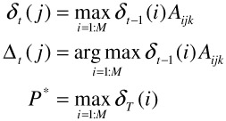
P* is the probability of the best sequence given the input and the parametric mapping A. We can then backtrack the best sequence Q* as follows

In the above algorithm, we have allowed the density of the duration of each decision state to be exponential. This may not be a valid assumption. To rectify this we now introduce the duration dependent input output Markov model (DDIOMM). Our approach in modeling duration in the DDIOMM is similar to that by Ramesh et al. [48].

This model, in its standard form, assumes that the probability of staying in a particular state decays exponentially with time. However, most audio-visual events have finite duration not conforming to the exponential density. Ramesh et al. [48] have shown that results can improve by specifically modeling the duration of staying in different states. In our current work, we show how one can enforce it in case of models like duration dependent IOMM.

Let us define a new mapping function A={A_ijkd}, i,j∈{l,.,M}, k ∈{1,.,N}, d ∈{1,.,D} where A_ijkd=P(q_t=j|q_t-1=I,d_t-1(i)=d,y_t=k). A can again be estimated from the training data by frequency counting. We now propose the algorithm to estimate the best decision sequence given A and the input sequence γ. Let

(2.6)

where Q_t indicates all possible decision sequences until time t-1 and d_t(i) indicates the duration in terms of discrete time samples for which the path has continued to be in the state q_t. This can be recursively computed as follows

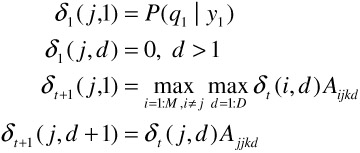
Let

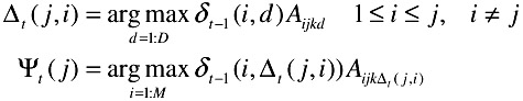
Finally

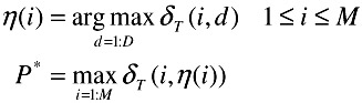
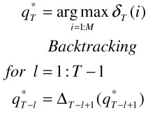
P* is the probability of the best sequence given the input and the parametric mapping A. We can then backtrack the best sequence Q* as follows

Backtracting

while t > 1

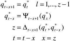
Using the above equations, one can decode the hidden state sequence. Each state or the group of states correspond to the state of the environment or the particular semantic concept that is being modeled. In the next section, we compare the performance of these models with the traditional HMMs and show that one can get huge improvements.