11.3 Domain-Independent Algorithms

11.3 Domain-Independent Algorithms

We discuss two families of domain-independent algorithms that have been used as the core of techniques for location prediction in mobile wireless systems.

11.3.1 The Order-K Markov Predictor

The order-k Markov predictor assumes that the next term of the movement history depends only on the most recent k terms. Moreover, the next term is independent of time, i.e., if the user's history consists of H_n = {X_l = a₁, ..., X_n = a_n}, then for all a ∈ A,

P(X_n+1 = a | H_n) = P(X_n+1 = a | X_n-k+1 = a_n-k+1, ..., X_n = a_n) = P(X_i+k+l = a | X_i+1 = a_n-k+1, ..., X_i+k = a_n), ∀i ∈ ℕ

The current state of the predictor is assumed to be < a_n-k+1, a_n-k+2, ..., a_n>.

If the movement history was truly generated by an order-k Markov source, then there would be a transition probability matrix M that encodes these probability values. Both the rows and columns of M are indexed by length-k strings from A^k so that P(X_n+1 = a | H_n) = M(s, s'), where s' and s are the strings a_n-k+1a_n-k+2...a_n and a_n-k+2a_n-k+3...a_na, respectively. In this case, knowing M would immediately provide the probability for each possible next term of H_n.

Unfortunately, even if we assume the movement history is an order-k Markov chain for some k we do not know M. Here is how the order-k Markov predictor estimates the entries of M. Let N(t, s) denote the number of times the substring t occurs in the string s. Then, for each a ∈ A,

(11.2)

If r predictions are allowed for X_n+1 then the predictor chooses the r symbols in A. with the highest probability estimates. In other words, the predictor always chooses the r symbols which most frequently followed the string a_n-k+1...a_n in H_n.

Vitter and Krishnan ^[16] suggested using the above predictor in the context of prefetching Web pages. Chan and coworkers ^[17] considered five prediction algorithms, three of which can be expressed as order-k predictors. (We will briefly describe the other two in a later section.) Two of them, the location based and direction-based prediction algorithms, are equivalent to the order-1 and order-2 Markov predictors, respectively, when A is the set of all cell IDs. The time-based prediction algorithm is an order-2 Markov predictor when A is the set of all time-cell ID pairs.

We emphasize that the above prediction scheme can be used even if the movement history is not generated by an order-k Markov source. If the assumption about the movement history is true, however, the predictor has the following nice property. Consider F, the family of prediction algorithms that make their decisions based only on the user's history, including those that have full knowledge of the matrix M. Suppose each predictor in F is used sequentially so that a guess is made for each X_i. We say that a predictor has made an error at step i if its guess does not equal X_i. Let , where I is the indicator function, denote the average error rate for the order-k Markov predictor. Let F(H_n) be the best possible average error rate achieved by any predictor in F. Vitter and Krishnan ^[18] showed that as n → ∞, , i.e., the average error rate of the order-k predictor is the best possible as, n → ∞, or that the average error rate is asymptotically optimal. This result holds for any given value of k.

We observe that the algorithm can (naively) be generalized for predicting location beyond the next cell, i.e., predicting the user's path, as follows. If M is known, P(X_t = a | H_n) for any t > n + 1 and each a ∈ A can be determined exactly from M^(t-n). The process to estimate M^(t-n) is to first construct , the estimate for M, and then raising it to the (t - n)th power. Then the value(s) of X_t can be predicted using the same procedure as for X_n+1. However, any errors in the estimate of M will accumulate as prediction is attempted for further steps in the future.

11.3.2 The LZ-Based Predictors

LZ-based predictors are based on a popular incremental parsing algorithm by Ziv and Lempel ^[19] used for text compression. Some of the reasons this approach was considered were (1) most good text compressors are good predictors ^[20] and (2) LZ-based predictors are like the order-k Markov predictor except that k is a variable allowed to grow to infinity. ^[21] We first describe the Lempel-Ziv parsing algorithm.

11.3.2.1 The LZ Parsing Algorithm

Let y be the empty string. Given an input string s, the LZ parsing algorithm partitions the string into distinct substrings s₀,s₁,...,s_m such that s₀=γ, for all j ≥ 1, substring S_j without its last character is equal to some s_i, 0 ≤ i < j, and s₀,s₁,...,s_m = s. Observe that the partitioning is done sequentially, i.e., after determining each s_i, the algorithm only considers the remainder of the input string. For example, H_n = abbbbdeeefffddddb is parsed as γ, a, b, bb, bd, e, ee, f, ff, d, dd, db.

Associated with the algorithm is a tree, which we call the LZ tree, that is grown dynamically to represent the substrings. The nodes of the tree represent the substrings where node s_i is an ancestor of node s_j if and only if s_i is a prefix of s_j. Typically, statistics are stored at each node to keep track of information such as the number of times the corresponding substring has been seen as a prefix of s₀,s₁,...,s_m or the sequence of symbols that has followed the substring. The tree associated with this example is shown in Figure 11.2.

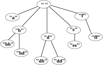
Figure 11.2: An example LZ parsing tree.

Suppose s_m+1 is the newest substring parsed. The process of adding the node corresponding to the s_m+1 in the LZ tree is equivalent to tracing a path starting from the root of the tree through the nodes that correspond to the prefixes of s_m+1 until a leaf is reached. The node for s_m+1 is then added to this leaf. Path tracing resumes at the root.^{[22],[23],[24],[25],[26],[27],[28]}

11.3.2.2 Applying LZ to Prediction

Different predictors based on the LZ parsing algorithm have been suggested in the past. ^[29],^[30],^[31],^[32],^[33],^[34],^[35],^[36], ^[37], ^[38], ^[39], ^[40] We describe some of these here and then discuss how they differ.

Suppose H_n has been parsed into s₀,s₁,...,s_m. If the node associated with s_m is a leaf of the LZ tree, then LZ-based predictors usually assume that each element in A is equally likely to follow s_m. That is, . Otherwise, LZ-based predictors estimate P(X_n+1 = a | H_n) based on the symbols that have followed s_m in the past when H_n was parsed.

1. Vitter and Krishnan ^[41] considered the case when the generator of H_n is a finite-state Markov source, which produces sequences where the next symbol is dependent on only its current state. (We note that a finite-state Markov source is more general than the order-k Markov source in that the states do not have to correspond to strings of a fixed length from A.) They suggested using the following probability estimates: for each a ∈ A, let

   (11.3)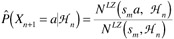

   

   where N^LZ(s',s) denotes the number of times s' occurs as a prefix among the substrings s₀,..., s_m, which were obtained by parsing s using the LZ algorithm.

   It is worthwhile comparing Equation 11.2 with Equation 11.3. While the former considers how often the string of interest occurs in the entire input string, (i.e., in our application, the history H_n), the latter considers how often it occurs in the partitions s_i created by LZ. Thus, in the example of Figure 11.2, while bbb occurs in H_n, it does not occur in any s_i.

   If r predictions are allowed for X_n+1, then the predictor chooses the r symbols in A that have the highest probability estimates. Once again, Vitter and Krishnan showed that this predictor's average error rate is asymptotically optimal when used sequentially.

2. Feder and coworkers ^[42] designed a predictor for arbitrary binary sequences, i.e., sequences where A= {0,1}. The following are their probability estimates:

   (11.4)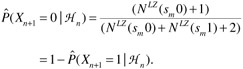

   

   For convenience let . Then the predictor guesses that the next term is 0 with probability φ/α, where for some chosen ε > 0

   

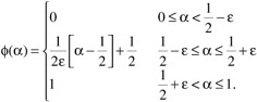
   Essentially, the predictor outputs 0 if a is above 1/2 + ε, 1 if α is below 1/2 + ε, and otherwise outputs 0 or 1 probabilistically.

   Example: Let s_m = 00 and suppose N^LZ(000) = 11 and N^LZ (001) = 9. Thus, . If ε =0.01, then the predictor would guess 0 for X_n+1; if ε =0.25, then the predictor would guess 0 for X_n+1 with probability of 13/22 and 1 with probability 9/22.

   Compare the output of Vitter and Krishnan ^[43] with Feder and coworkers' algorithm ^[44] for this example assuming a single prediction is desired (r = 1). The former simply calculates the probability estimates , so that the prediction is 0. The latter provides predictions with certainty only if the probability estimates for 0 and 1 are not too close (i.e., not within 2ε of each other).

   If the predictor is used sequentially, then Feder and coworkers ^[45] showed that its asymptotic error rate is the best possible among predictors with finite memory.

3. Krishnan and Vitter generalized Feder and coworkers' procedure and result to arbitrary sequences generated from a bigger alphabet; ^[46] i.e., |A| ≥ 2. Their scheme for computing for each a ∈ A is not only based on how frequently a followed s_m, but also on the order in which the symbols followed s_m. Specifically, they assigned probability estimates in the following manner. Suppose after the first occurrence of s_m, the next occurrence is s_mh₁ for some symbol h_l, the following occurrence is s_mh₂, etc. Consider all the symbols h_i that have followed s_m (after its first occurrence), and create the sequence h = h₁h₂h...h_t. Let h(i, j) denote the subsequence h_ih_i+1h...h_j. Let and h'= h(4q^-1 + 2, t). Then for each a ∈ A,

   (11.5)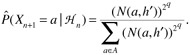

   

   If r predictions are allowed for X_n+1, then the predictor uses these probability estimates to choose without replacement r symbols from A

   Example: Suppose 9 symbols from A = {0,1,2} followed s_m and the sequence of the symbols is h = 210011102. Thus, q = 2. The relevant subsequence h for predicting X_n+1 is 1102. The frequency of 0, 1, and 2 in the subsequence are 1, 2, and 1, respectively, so their probability estimates are 1/18, 16/18, and 1/18, respectively. The predictor will pick r of these symbols without replacement using these probabilities

4. Bhattacharya and Das ^[47] proposed a heuristic modification to the construction of the LZ tree, as well as a way of using the modified tree to predict the most-likely cells that the user will reside in so as to minimize paging costs to locate the user. The resulting algorithm is called LeZi-Update. Although their application (similar to that of Yu and Leung ^[48]) lies in the mobile wireless environment, the core prediction algorithm itself is not specific to this domain. For this reason, and for ease of exposition, we include it in this section.

   As pointed out earlier, not every substring in H_n forms a leaf s_i in the LZ parsing tree. In particular, substrings that cross boundaries of the s_i, 0 < i ≤ m, are missed. Further, previous LZ-based predictors take into account only the occurrence statistics for the prefixes of the leaves s_i. To overcome this, the following modification is proposed. When a leaf s_i is created, all the proper suffixes of s_i are considered (i.e., all the suffixes not including s_i itself.) If an interior node representing a suffix does not exist, it is created, and the occurrence frequency for every prefix of every suffix is incremented.

   Example: Suppose the current leaf is s_m = bde and the string de is one that crosses boundaries of existing s_i for 1 ≤ i < m (see Figure 11.2). Thus de has not occurred as a prefix or a suffix of any s_i, 0 < i < m. The set of proper suffixes of s_m is S_m = {γ,e,de} and because there is no interior node for de, it is created. Then the occurrence frequency is incremented for the root labeled _γ, the first-level children b and d, and the new interior node de.

   We observe that this heuristic only discovers substrings that lie within a leaf string. Also, at this point it would be possible to use the modified LZ tree and apply one of the existing prediction heuristics, e.g., use Equation 11.3 and the Vitter-Krishnan method.

   However, in Bhattacharya and Das ^[49] a further heuristic is proposed to use the modified LZ tree for determining the most-likely locations of the user. This second heuristic is based on the prediction by partial match (PPM) algorithm for text compression. ^[50] (The PPM algorithm essentially attempts to "blend" the predictions of several order-k Markov predictors, for k = 1, 2, 3, ...; we do not describe it here in detail.) Given a leaf string s_m, the set of proper suffixes S_m is found. Observe that each element of S_m is an interior node in the LZ tree. Then, for each suffix, the heuristic considers the subtree rooted at the suffix and finds all the paths in this subtree originating from the root. (Thus these paths would be of length l for l = 1, 2,...t, where t is the height of the suffix in the LZ tree.) The PPM algorithm is then applied. PPM first computes the predicted probability of each path in the entire set of paths and then uses these probabilities to compute the most-probable symbol(s), which is the predicted location of the user.

5. Yu and Leung ^[51] use LZ prediction methods for call admission control and bandwidth reservation. Their mobility prediction approach is novel in that it predicts both the location and handoff times of the users. Assume time is discretized into slots of a fixed duration. The movement history H_n of a user is recorded as a sequence of ordered pairs (S,l₁),(T₂,l₂),...,(T_n,l_n), where S is the time when the call was initiated at cell l₁ and S + T_i is when the i-th handoff occurred to cell l_i for i ≥ 2. In other words, T_i is the relative time (in time slots) that has elapsed since the beginning of the call when the i-th handoff was made.

   Similar to LeZi-Update, if the user is currently at cell l and time S + T, the predictor uses the LZ tree to determine the possible paths the user might take and then computes the probabilities of these paths. Unlike LeZi-Update, the computation is easier and is not based on PPM. The algorithm estimates the probabilities P_i,j(T_k), the probability that a mobile in cell i will visit cell j at timeslot S + T_k, by adding up the probabilities of the paths in the LZ tree that are rooted at the current time-cell pair and contain the ordered pair (j, T_k).

11.3.3 Other Approaches

Chan et al. ^[52] suggest a different approach for location prediction based on using an order-2 Markov predictor with Bayes' rule. The idea is to first predict the general direction of movement and then use that to predict the next location. For the order-2 predictor, the last two terms of the user's itinerary, L = <L₁, L₂> are used. First, the most-likely location m steps away from the current location, i.e., L_2+m, is predicted based on the user's past history. Then the next location L₃ is predicted using Bayes' rule and the reference point L_m+2 by choosing the location B_x with the highest probability as follows.

(11.6)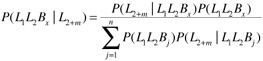

^[16]Vitter, J. and Krishnan, P., Optimal prefetching via data compression, J. ACM, 43 (5), 771–793, 1996.

^[17]Chan, J., Zhou, S., and Seneviratne, A., A QoS adaptive mobility prediction scheme for wireless networks, Proc. IEEE Globecom, Sydney, Australia, Nov. 1998.

^[18]Vitter, J. and Krishnan, P., Optimal prefetching via data compression, J. ACM, 43 (5), 771–793, 1996.

^[19]Ziv, J. and Lempel, A., Compression of individual sequences via variable-rate coding, IEEE Trans. Inf. Theory, 24 (5), 530–536, 1978.

^[20]Vitter, J. and Krishnan, P., Optimal prefetching via data compression, J. ACM, 43 (5), 771–793, 1996.

^[21]Bhattacharya, A. and Das, S.K., LeZi-update: an information-theoretic framework for personal mobility tracking in PCS networks, ACM/Kluwer Wireless Networks, 8 (2–3), 121–135, 2002.

^[22]Chan, J. et al., A framework for mobile wireless networks with an adaptive QoS capability, Proc. Mobile Mult. Comm. (MoMuC), Oct. 1998, pp. 131–137.

^[23]Erbas, F. et al., A regular path recognition method and prediction of user movements in wireless networks, IEEE Vehic. Tech. Conf. (VTC), Oct. 2001.

^[24]Levine, D., Akyildiz, I., and Naghshineh, M., A resource estimation and call admission algorithm for wireless multimedia networks using the shadow cluster concept, IEEE/ACM Trans. Networking, 2, 1–15, 1997.

^[25]Bharghavan, V. and Jayanth, M. Profile-based next-cell prediction in indoor wireless LAN, Proc. IEEE SICON, Singapore, Apr. 1997.

^[26]Riera, M. and Aspas, J., Variable channel reservation mechanism for wireless networks with mixed types of mobility platforms, Proc. IEEE Vehic. Tech. Conf. (VTC), May 1998, pp. 1259–1263.

^[27]Oliveira, C., Kim, J., and Suda, T., An adaptive bandwidth reservation scheme for high-speed multimedia wireless networks, IEEE J. Selected Areas Commun., 16 (6), 858–874, 1998.

^[28]Chua, K.C. and Choo, S.Y., Probabilistic channel reservation scheme for mobile pico/microcellular networks, IEEE Commun. Lett., 2 (7), 195–196, 1998.

^[29]Yu, F. and Leung, V., Mobility-based predictive call admission control and bandwidth reservation in wireless cellular networks, Computer Networks, 38, 577–589, 2002.

^[30]Posner, C. and Guerin, R., Traffic policies in cellular radio that minimize blocking of handoff calls, Proc. 11th Int. Teletraffic Cong., Kyoto, Japan, 1985.

^[31]Ramjee, R., Nagarajan, R., and Towsley, D., On optimal call admission control in cellular networks, Proc. IEEE Infocom, San Francisco, 1996.

^[32]Naghshineh, M. and Schwartz, M., Distributed call admission control in mobile/wireless networks, IEEE J. Selected Areas Commun., 14, 711–717, 1996.

^[33]Chao C. and Chen, W. Connection admission control for mobile multiple-class personal communications networks, IEEE J. Selected Areas Commun., 15, 1618–1626, 1997.

^[34]Luo, X., Thng, I., and Zhuang, W., A dynamic channel pre-reservation scheme for handoffs with GoS guarantee in mobile networks, Proc. IEEE ICC, Vancouver, Canada, 1999.

^[35]Zhang, T. et al., Local predictive reservation for handoff in multimedia wireless IP networks, IEEE J. Selected Areas Commun., 19, 1931–1941, 2001.

^[36]Bharghavan, V. et al., The TIMELY adaptive resource management architecture, IEEE Pers. Commun., 20–31, 1998.

^[37]Bhattacharya, A. and Das, S.K., LeZi-update: an information-theoretic framework for personal mobility tracking in PCS networks, ACM/Kluwer Wireless Networks, 8 (2–3), 121–135, 2002.

^[38]Vitter, J. and Krishnan, P., Optimal prefetching via data compression, J. ACM, 43 (5), 771–793, 1996.

^[39]Krishnan, P. and Vitter, J., Optimal prediction for prefetching in the worst case, SIAM J. Computing, 27 (6), 1617–1636, 1998.

^[40]Feder, M., Merhav, N., and Gutman, M., Universal prediction of individual sequences, IEEE Trans. Inf. Theory, 38, 1258–1270, 1992.

^[41]Vitter, J. and Krishnan, P., Optimal prefetching via data compression, J. ACM, 43 (5), 771–793, 1996.

^[42]Feder, M., Merhav, N., and Gutman, M., Universal prediction of individual sequences, IEEE Trans. Inf. Theory, 38, 1258–1270, 1992.

^[43]Vitter, J. and Krishnan, P., Optimal prefetching via data compression, J. ACM, 43 (5), 771–793, 1996.

^[44]Feder, M., Merhav, N., and Gutman, M., Universal prediction of individual sequences, IEEE Trans. Inf. Theory, 38, 1258–1270, 1992.

^[45]Feder, M., Merhav, N., and Gutman, M., Universal prediction of individual sequences, IEEE Trans. Inf. Theory, 38, 1258–1270, 1992.

^[46]Krishnan, P. and Vitter, J., Optimal prediction for prefetching in the worst case, SIAM J. Computing, 27 (6), 1617–1636, 1998.

^[47]Bhattacharya, A. and Das, S.K., LeZi-update: an information-theoretic framework for personal mobility tracking in PCS networks, ACM/Kluwer Wireless Networks, 8 (2–3), 121–135, 2002.

^[48]Yu, F. and Leung, V., Mobility-based predictive call admission control and bandwidth reservation in wireless cellular networks, Computer Networks, 38, 577–589, 2002.

^[49]Bhattacharya, A. and Das, S.K., LeZi-update: an information-theoretic framework for personal mobility tracking in PCS networks, ACM/Kluwer Wireless Networks, 8 (2–3), 121–135, 2002.

^[50]Bell, T.C., Cleary, J.G., and Witten, I.H., Text Compression, Prentice Hall, New York, 1990.

^[51]Yu, F. and Leung, V., Mobility-based predictive call admission control and bandwidth reservation in wireless cellular networks, Computer Networks, 38, 577–589, 2002.

^[52]Chan, J., Zhou, S., and Seneviratne, A., A QoS adaptive mobility prediction scheme for wireless networks, Proc. IEEE Globecom, Sydney, Australia, Nov. 1998.