Cells and Ranges

---

At the bottom of the organizational hierarchy in Excel is the cell, which is formed by the intersection of a column and a row in a worksheet. A cell can contain a value or a formula. By default, Excel displays the result of a formula in its cell, but you can change that setting by clicking Tools, Options, clicking the View tab, and selecting Formulas. What’s interesting is that the formula in a cell is always displayed in the formula bar, regardless of whether or not you have formulas displayed in the cells. You might expect Excel to toggle between showing the formula result or the formula based on what was shown in the body of the worksheet.

Note 

Displaying formulas instead of the formulas’ results in a worksheet’s cells displays the Formula Auditing toolbar, which has buttons you can use to identify cells used in your formulas, watch how the values in specific cells change, and step through formulas one calculation at a time to zero in on errors.

After you have your data, you can choose how to display it. The Formatting toolbar, which is displayed by default, has a range of buttons you can use to make basic changes to the appearance of your data, such as displaying the cell’s contents in bold type or in a different font, but if you want fine control over your data’s appearance you need to click Format, Cells to display the dialog box shown in Figure 2-2. From within the Format Cells dialog box, you can change the direction of the text in a cell, cause the contents of a cell to shrink to fit the existing size of the cell without wrapping, or add borders to a cell. It can be easy to go overboard with the formatting, so you should always keep in mind that the objective of an Excel worksheet is to make the data easy to read, not to display it as a work of art.

Figure 2-2: Use the controls in the Format Cells dialog box to present your data effectively.

You can deal with cells individually or in groups. When you want to change the formatting of a group of cells, you can select the cells and make any changes you desire. If you want to use the values from a group of cells in a formula, you can do much the same thing. For example, you could type a formula such as =SUM() into a cell, set the insertion point between the parentheses, and then select the cells you want to be used in the formula. As you select cells, the cell references are inserted into the formula. In this instance, selecting the cells from C3 to C24 would result in the formula =SUM(C3:C24). And, as of Excel 2002, you are able to select discontiguous groups of cells by holding down the Ctrl key. For example, typing =SUM() into a cell, positioning the insertion point between the parentheses, selecting cells C3 to C24, and then holding down the Ctrl key while you select cell C26, would result in the formula =SUM(C3:C24,C26).

Important 

When creating a formula, pressing the Enter key before you complete the formula will result in an error. You need to type =SUM( and then select the cells you want to include, before you type the closing parenthesis.

When you work with a lot of worksheets and formulas, or if you need to pass a workbook you created to a colleague, just using cell references to designate the values used in a formula can lead to a lot of confusion. Rather than stay with the simple but somewhat cryptic cell references, you can create named ranges (often just called names) to make your formulas easier to read. For example, if you had a worksheet with sales for several different product categories, you could create a named range for each category and create a formula such as =SUM(MachineTools,Software,Consulting) instead of =SUM(C3:C24,D3:D24,E3:E24).

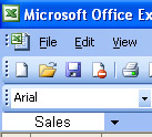
The quickest way to create a named range is to select the cells you want in the range, click in the Name box at the left edge of the formula bar, and type the name for the range. (The Name box is the area in the formula bar that displays the address of the currently selected cell.)

If you want to work with existing ranges, you can click Insert, Name, Define to display the Define Name dialog box, shown in Figure 2-3. From there, you can add or delete ranges.

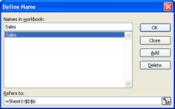
Figure 2-3: Use the Define Name dialog box to manage your named ranges.

You can have Excel show which cells comprise a named range by clicking the down arrow at the right edge of the Name box and clicking the name of the range you want to see.

---