9.7 Generalized Petri nets

---

9.7 Generalized Petri nets

Generalized Petri nets are used to provide yet another refinement of the models discussed up to this point. All of the other models had transitions, which, when fired, either were performed instantaneously or within some pre-described time period. The time period for a transition's firing, once set, was fixed and did not change over the course of the model's lifetime. This is adequate if we have deterministic timing in our modeled system and there is no variability. In reality we know this does not hold for most realistic systems. Generalized Petri net models alter this by providing mechanisms for associating a random, exponentially distributed firing delay with timed transitions.

The addition required to meet these new conditions for firing is a function defined over transitions in the system. This new function is called rate or weight transition function. This function, W(t_k, μ), must be defined for each transition and state in the network. If the function does not need to be defined for all markings, then we can simply refer to the function as W(t_k), where t_k ∈ T. The result of this function, W(t_k, μ) or W(t_k), is called the rate of transition t_k in marking μ if t_k is timed and the weight of transition t_k in marking μ if t_k is immediate. The value of this result is a random variable defined by the exponential function defined for the transition around the selected mean value.

Firing of a transition in a generalized net occurs as in a timed net except that the time to fire the transition is computed using an exponential function defined around a mean value. Each transition in the net must have a rate, r, defined for it. The rate is the mean value for use in computing the actual time to use in firing the transition. Once a transition is enabled, its computed timer value is decremented using a system-determined increment value until it either reaches 0 or it loses its enabling tokens. As in the timed net, we can use additional information or policies to decide how to use the state of the transition when it becomes nonenabled. We could use the remaining time in the computed time, reset the same time, or select another new time based on the same mean. All have merits based on the type of element being modeled.

Another difference in this class of system is the concept of system state. The state of the system changes from one state to another state based on the firings of all active and ready transitions during this present time interval. In Figure 9.30, the initial marking is (μ₀ = (2,0,0). If we use the colored net functions and simply change the transition times into rates, we now have a generalized Petri net. In the example, transition t₁, once enabled, will compute a transition rate using the mean rate, r₁, as the value fed into the negative exponential. Using the computed rate the timer would initiate decrements until it reached the firing point (timer value = 0). We would then use the selected token to determine which path to choose in leaving the transition. In the example, if the choice function chose white, then we would take the white path, resulting in a new system state, μ₁ = (1,0,1).

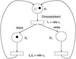
Figure 9.30: Generalized Petri Net.

An important concept with these nets is that they would not compute the same state each time they executed from a given state, due to the randomness of the possible transition firing time. This is a desirable feature for such models, as it was when we used this same property for the memoryless property for arrival rates and service rates at queues.

---