Chapter 5: Probability
|
| < Free Open Study > |
|
Overview
Queuing theory and queuing analysis are based on the use of probability theory and the concept of random variables. We utilize the concepts embodied in probability in a number of different ways. For example, we may ask what the probability is of the Boston Bruins winning the Stanley Cup this year. How likely is George W. Bush to be reelected after the events of this year? How likely is it to snow on the top of Mt. Washington in New Hampshire in January of this year? Most of the time a general answer would suffice. For example, it is highly probable that snow will fall sometime in January on Mt. Washington. Conversely, based on the last 30 years of frustration, it is also highly unlikely that the Boston Bruins will win the Stanley Cup this year. Probability theory allows us to make more precise definitions for the probability of an event occurring based on past history or on specific available measurements, as we will see. In this chapter, we will introduce the concepts of probability, joint probability, conditioned probability, and independence. We will then move on to probability distributions, stochastic processes, and, finally, the basics of queuing theory.
Before discussing queuing analysis, it is necessary to introduce some concepts from probability theory and statistics. In basic probability theory, we start with the ideas of random events and sample spaces. Take, for instance, the experiment that involves tossing a fair die (an experiment typically defines a procedure that yields a simple outcome, which may be assigned a probability of occurrence). The sample space of an experiment is simply the set of all possible outcomes-in this case the set {1,2,3,4,5,6} for the die. An event is defined as a subset of a sample space and may consist of none, one, or more of the sample space elements. In the die experiment, an event may be the occurrence of a 2 or that the number that appears is odd. The sample space, then, contains all of the individual outcomes of an experiment. For the previous statement to hold, it is necessary that all possible outcomes of an experiment are known.
The fundamental tenet of probability states that the chance of a particular outcome occurring is determined by the ratio of the number of favorable outcomes (successes) to the total number of outcomes (the sample space). Expressed as a formula for some event, A:
| (5.1) |
From the previous example, the probability of rolling a 2, stated as P(2), using a fair die, is equal to the ratio 1/6 or 0.167. In this experiment, 1 represents the favorable outcome or success of our experiment, and 6 represents the total number of possible outcomes from rolling the die. Likewise, we could determine the probability of rolling an odd number (1, 3, or 5) stated as P(odd), as 3/6 or 0.5. In this experiment, 3 represents the number of possible outcomes that represent favorable outcomes for this experiment, and 6 represents the total number of possible outcomes from rolling the die. Another example using playing cards may further refine this definition. If we have a well-shuffled deck of cards with 52 possible cards that could be drawn, and we wish to know the probability of drawing a king, this could be stated as:
| (5.2) | 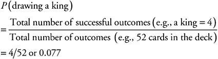 |
One could ask the probability of drawing the king of hearts as:
| (5.3) | 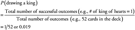 |
In all cases, the value for the probability of an event occurring within a range of all possible events must span from 0, where the event does not occur (e.g., rolling a zero with a die; since there are no zeros on the die, this is not possible) to a maximum of 1 (e.g., the probability of rolling an odd or even number with the die) indicating the event always occurs.
In the examples cited, each number on the die must have an equal chance of being rolled. Likewise, in the cards example, each card must have an equal chance of being drawn. No number on the die face or card in the deck can be differentiated so that it would be more likely to be chosen or rolled (e.g., a weighted die is not a fair die).
The theory of probability was constructed based on the concept of mutual exclusion (disjointedness) of events. That is, events cannot occur at the same time in an experiment if they are mutually exclusive. For example, the rolling of the fair die can result in one of six possible outcomes, but not two or more of them at the same time. A second example is a fair coin-flipping the coin will result in a head or tail being displayed but not both a head and tail. Therefore, the outcome of the event rolling a die and getting a 1 versus all other numbers is said to be mutually exclusive, as is the flipping of the coin resulting in either the head or tail but not both.
Another important property within the field of probability is that of independence. For example, if we have a coin and a die, we intuitively understand that the event of flipping the coin and rolling the die have independent outcomes. That is, the result of one will not affect the outcome of the other. The sample space for the two events is composed of the Cartesian product of the two independent spaces; since all events of both are independently possible, the resulting sample space must include all possible combinations of the two independent spaces.
If we believe that this property of equal likelihood exists, then the probability of any of these outcomes must be equal and composed of the multiplicative probability of each independently. In the previous example, the fair coin flip has a sample space consisting of the elements of the set {H,T}, each with a probability of 1/2, and the fair die has a sample space consisting of the elements of the set {1,2,3,4,5,6}, each with a probability of 1/6. The probability of the combination of either of these events occurring would be derived from the Cartesian product set {H1,H2,H3,H4,H5,H6,T1,T2,T3,T4,T5,T6}, with any of these combined events, yielding an equal probability equal to 1/2 × 1/6, or 1/12.
In general, when events are independent, sample spaces where each event occurs are equally likely. If there are n1 items in the first event space, n2 in the second, and nm in the last sample space, then the sample space of the combined events space is equal to the sum of the size of each of these spaces:
| (5.4) |
The probability of any individual event occurring is then equal to 1/(n1 + n2 + ... + nm), which, in the previous example, was found to be 1/12.
We will not always be interested in the likelihood of just one event from a total sample space occurring but rather some subset of events from the total space. For example, we may be interested in the likelihood of only one head occurring during the flipping of four coins. The complete sample space for this experiment has exactly 16 possible outcomes:
{HHHH,HHHT,HHTH,HTHH,THHH,TTHH,THHT,HHTT,THTH,HTHT,HTTH, HTTT,THTT,TTHT,TTTH,TTTT} From this space, we can see that the events meeting the desired outcome of only one head results in the subset:
{HTTT,THTT,TTHT,TTTH} where each item in this subset is equally likely to occur from the original set, so each has the equal probability of 1/16. Their combined probability would represent the desired probability of only one head occurring and would be equal to the sum of their probability: 4/16 or 1/4. In this example, we are using the additive probabilities of these events to see the likelihood of one of these occurring from the original set. To compute the subset probability we need only know the size of the original set and the size of the subset.
More often, we are faced with the problem of determining the possibility of some event occurring given that some prior event has already occurred. For example, we may be asked the probability of our computer system failing given that one memory chip has failed. This concept of related or dependent events is called conditional probability. The effect of applying this property to two independent event spaces is to remove some of the possible combinations from the final combined space of possible values. For example, we may be asked what the probability is of getting exactly one head after the first element was found to be a tail in the four-coin toss. The initial sample space was 16, but given that we removed the events where the initial toss resulted in a tail, the resultant space now has only eight possible outcomes and from these there are only three within the sub-space meeting our final desired outcome.
To compute what the probability is in this case, we can do a few things. First, we can compute the probability of realizing the tail on the first toss as 8/16 and the probability that there is one head from the last three tosses as 3/8. Many times it is easier to compute the opposite occurrence. That is, let's compute the probability that the final event does not happen. First, we may reason that the sample space now excludes all events where the first item was a head, or eight events. There are now only 16 - 8 or 8 equally likely events remaining in our space. Of these remaining 8, there are five ways in which, given a tail first, we do not get exactly one head. The probability of at least one head is then the ratio of the number of successes (3) to the total number of possible events (16 - 8) or 8, resulting in a probability of 3/8.
Several operations on the events in the sample space yield important properties of events. By definition, the intersection of two events is the set that contains all elements common to both events. The intersection of sets A and B is written AB. By extension, the intersection of several events contains those elements common to each event. Two events are said to be mutually exclusive if their intersection yields the null set. The union of two events yields the set of all of the elements that are in either event or in both events. The union of sets A and B is written A ⋃ B.
The complement of an event, denoted Ā, represents all elements except those defined in the event A. The following definition, known as DeMorgan's Law, is useful for relating the complements of two events:
| (5.5) |
Permutations and combinations of elements in a sample space may take many different forms. Often, we can form probability measures about combinations of sample points, and the basic combinations and permutations discussed in the following text are of use in this task. By definition, a combination is an unordered selection of items, whereas a permutation is an ordered selection of items. The most basic combination involves the occurrence of one of n1 events, followed by one of n2 events, and so on to one of nk events. Thus, for each path taken to get to the last event, k, there are nk possible choices. Backing up one level, there were nk-1 choices at that level, thereby yielding nk-1nk choices for the last two events. Following similar logic backing up to the first level yields:
| (5.6) | 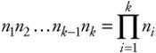 |
possible paths. For example, in a string of five digits, each of which may take on the values 0 through 9, there are 10 × 10 × 10 × 10 × 10 = 100,000 possible combinations, or nk possible outcomes, where n = 10 and k = 5 in the sample space. The assumption is that once an item has been sampled, it is returned to the space for possible resampling. This is sometimes referred to as sampling with replacement. The probability distribution for a random selection of items is uniform; therefore, each item in the sample space will have the probability of 1/nk.
When dealing with unique elements that may be arranged in different ways, we speak of permutations. When we have n things and sample n times, but do not replace the sample items before the next selection, we now have a selection without replacement, also referred to as a permutation. For n distinct objects, if we choose one and place it aside, we then have n - 1 left to choose from. Repeating the exercise leaves n - 2 to choose from, and so on down to 1. The number of different permutations of these n elements is the number of choices you can make at each step in the select and put aside process and is equal to:
| (5.7) |
The common notation P(n,k) denotes the number of permutations of n items taken k at a time. To find the numerical value for a random selection we can use similar logic. The first item may be selected in n ways, the second in n - 1 ways, the third in n - 2 ways, and the kth or last item we choose in n - k - 1 ways. Choosing from n distinct items taken in groups of k at a time yields the following number of permutations or product space for this experiment:
| (5.8) |
The permutation yields the number of possible distinct groups of k items when picked from a pool of n. We can see that this is the more general case of the previous expression and reduces to equation (5.7) when k = n (also, by definition, 0! = 1). For example, if we wished to see how many ways we could arrange three computer servers on a workbench of five distinct servers, we would assume that the order of the servers has some meaning; therefore, we have:
| (5.9) |
A combination is a permutation when the order is ignored. One special case occurs when there are only two kinds of items to be selected. These are called binomial coefficients or C(n,k). The number of combinations of n items taken k at a time (denoted C[n,k]) is equivalent to P(n,k) reduced by the total number of k element groups that have the same elements but in different orders (e.g., P[k,k]). This is intuitively correct, because order is unimportant for a combination, and, hence, there will be fewer unique combinations than permutations for any given set of k items. P(k,k) is given in equation (5.7), hence:
| (5.10) |
Alternatively, one can state that each set of k elements can form P(k,k) = k! permutations, which, when multiplied by C(n,k), yields P(n,k). Dividing by P(k,k) yields:
| (5.11) |
| (5.12) |
Now that we have characterized some of the ways that we can construct sample spaces, we can determine how to apply probabilities to the events in the sample space. The first step to achieving this is to assign a set of weights to the events in the sample space. The choice of which weighting factor to apply to which event in the sample space is not an easy task. One method is to employ observations over a sufficiently long period so that a large sample of all possible outcomes is obtained. This is the so-called "observation, deduction, and prediction cycle," and it is useful for developing weights for processes where an underlying model of the process either does not exist or is too complex to yield event weights. This method, sometimes called the "classical probability definition," defines the probability of any event as the following:
| (5.13) |
where P(A) denotes the probability of event A, NA is the total number of observations where the event A occurred, and N is the total number of observations made. An extension to the classical definition, called the "relative frequency definition," is given as:
| (5.14) |
The preceding two approaches, combinations/permutations and relative frequency, are often used in practice as a means of establishing a hypothesis about how a process behaves. These methods do indeed define hypotheses because they are both based on the observation of a finite number of observations. This fact drives the desire to develop axiomatic definitions for the basic laws of probability.
Probability theory, therefore, is based upon a set of three axioms. By definition, the probability of an event is given by a positive number. That is:
| (5.15) |
The following relationship is also defined:
| (5.16) |
That is, the sum of all of the probabilities of all of the events in the total sample space S is equal to 1. This is sometimes called the "certain event." The previous two definitions represent the first two axioms and necessarily restrict the probability of any event to between 0 and 1 inclusively. The third is based on the property of mutual exclusion, which states that two events are mutually exclusive if, and only if, the occurrence of one of the events positively excludes the occurrence of the other. In set terminology, this states that the intersection of the two events contains no elements; that is, it is the null set. For example, the two events in the coin-toss experiment (heads and tails) are mutually exclusive. The third axiom, then, states that the combined probability of events A or B occurring is equal to the sum of their individual probabilities. That is:
| (5.17) |
So, for example, the probability of a head being tossed or a 6 being rolled is equal to the probability of a head being tossed or 1/2, plus the probability of rolling a 6, or 1/6, which is 4/6.
The reader is cautioned that the expression to the left of the equal sign reads the probability of event A or event B, whereas the right-hand expression reads the probability of event A plus the probability of event B. This is an important relationship between set theory and the numerical representation of probabilities.
The three axioms of probability are as follows:
| (5.18) |
| (5.19) |
| (5.20) |
In equation (5.20), the terminology AB is taken as the set A intersected with the set B. The sample space is defined on the total set {A1 ... Ak} as:
| (5.21) |
A very important topic in probability theory is that of conditional probability. Consider the following experiment in which we have the events A, B, and AB. For example, a disk crash and a memory failure could be event A and B, respectively, and a disk and memory failure at the same time is event AB. The event AB contains the events that are in A and B. Let us say that this event (AB) occurs NAB times. Let NB denote the number of times event B occurs on its own. If we want to know the relative frequency of event A given that event B occurred, we could do the following experiment and computation:
| (5.22) |
That is, if both events A and B occur (event AB), the number of times event A occurs when event B also occurs is found as a fraction of the space of event B where event A intersects (see Figure 5.1). The notation for this relative frequency is denoted P(A|B) and reads as the conditional probability of event A given event B also occurred. If we form the following expression from equation (4.16):
| (5.23) |
Figure 5.1: Conditional probability space Venn diagram.
and apply equation (5.14), we obtain the traditional conditional probability definition:
| (5.24) |
One interesting simplification of equation (5.23) occurs when event A is contained in, or is a subset of, event B, so that AB = A. In this case, equation (5.23) becomes:
| (5.25) |
Two events, A and B, are independent if their Venn diagrams do not intersect. The independence of two events is defined by the following formula:
| (5.26) |
or
| (5.27) |
This definition states that the relative number of occurrences of event A is equal to the relative number of occurrences of event A given event B occurred. In simpler terms, the independence of two or more events indicates that the occurrence of one event does not allow one to infer anything about the occurrence of the other.
Bayes's theorem is stated as follows: If we have a number of mutually exclusive events, B1, B2 ... BN, whose union defines the event space (or, more formally, a subset of the sample space), for some experiment, and an arbitrary event A from the sample space, the conditional probability of any event Bk in the set B1, B2 ... BN, given that event A occurs, is given by:
| (5.28) | 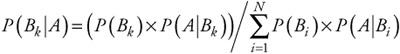 |
This result is an important statement, because it relates the conditional probability of any event of a subspace of events relative to an arbitrary event of the sample space to the conditional probability of the arbitrary event relative to all of the other events in the subspace. The theorem is a result of the total probability theorem, which states that:
| (5.29) |
The theorem holds because the events B1 ... Bk are mutually exclusive, and, therefore, event A = AS = A(B1, B2, ... Bk) = AB1 + AB2 + ... ABk ... so that:
| (5.30) |
Since events B1, B2 ... Bk are mutually exclusive, so are events AB1, AB2, ... ABk. Applying the conditional probability definition of equation (5.24) to equation (5.30) yields equation (5.28).
One other relationship that is often useful when examining conditional probability of two events is the following:
| (5.31) |
This formula states that for any two events, A and B, if we wish to determine if event A or B occurred or that both occurred, we need to examine them in isolation and in unison. This follows from the discussions of sets of events earlier in this chapter. Since the union of the events A and B yields all sample points in A and B considered together, the sum of the events separately will yield the same quantity plus an extra element for each element in the intersection of the two events. Thus, we must subtract the intersection to form the equality, hence equation (5.30). Note that equation (5.31) is essentially an extended version of equation (5.20), where AB does not equal the null set.
|
| < Free Open Study > |
|
EAN: 2147483647
Pages: 136