4.1 Scheduling algorithms
|
| < Free Open Study > |
|
4.1 Scheduling algorithms
When analyzing computer systems one ultimately must look at the scheduling algorithms applied to resource allocation. The means by which resources are allocated and then consumed are of utmost importance in assessing the performance of a computer system. For example, scheduling algorithms are applied when selecting which program runs on a CPU, what I/O device is serviced, and when or how a specific device handles multiple requests. When examining scheduling algorithms, two concepts must be addressed. The first is the major job of the scheduling algorithm, which is what job to select to run next. The second is to determine if the job presently running is the most appropriate to run and if not, should it be preempted (removed from service).
The most basic form of scheduling algorithm is first-come first-served (FCFS). In this scheduling algorithm jobs enter the system and get operated on based on their arrival time. The job with the earliest arrival time gets served next. This algorithm does not apply preemption to a running job, since the running job would still hold the criterion of having the earliest arrival time. A scheduling algorithm that operates opposite from the FCFS is the last-come first-served (LCFS) algorithm. In this algorithm the job with the most recent time tag is selected for operation. Given this algorithm's selection criteria, it is possible that this algorithm could be preemptive. The job being serviced is no longer the last to come in for service. The preemption decision must be made based on the resource's ability to be halted in midstream and then restarted at some future time. Processors typically can be preempted, since there are facilities to save registers and other information needed to restart a job at some later time. Other devices, such as a disk drive or I/O channel, may not have the ability to halt a job and pick it up at some later point.
A number and variety of scheduling algorithms are associated with processor scheduling. One of the most common processor scheduling algorithms is round robin. Round-robin scheduling is a combination algorithm. It uses FCFS scheduling, along with preemption. The processor's service is broken into chunks of time called quantum. These quanta or time slices are then used as the measure for service. Jobs get scheduled in an FCFS fashion as long as their required service time does not exceed the time of a quantum. If their required service time exceeds this, the job is preempted and placed in the back of the set of pending jobs. This motion of placing a job back into the FCFS scheduling pipe continues until the job ultimately completes. Thus, the job's service time is broken up into some number of equal, fixed-size time slices. The major issue with round-robin scheduling is the selection of quantum size. The reason quantum size selection is so important is due to the nature of preemption. Preempting a job requires overhead from the operating system to stop the job, save its state, and install a new job. If the time for these tasks is large in comparison to the quantum size, then performance will suffer. Many different rules of thumb have been developed in designing such systems. Most look to make the overhead a very small fraction of the size of the quantum-typically, orders of magnitude smaller. A method used for approximating round-robin scheduling when the quantum is very large compared with the overhead is processor sharing (PS). This model of round-robin scheduling is used in theoretical analysis, as we will see in later chapters.
Another algorithm is shortest remaining time first (SRTF). In this algorithm the job that requires the least amount of resource time is selected as the next job to service. The CPU scheduling algorithm SRTF does support preemption. When an arriving job is found to have a smaller estimated execution time than the presently running job, the running job is preempted and replaced by the new job. The problem with this scheduling algorithm is that one must know the processing requirements of each job ahead of time, which is typically not the case. Due to this limitation it is not often used. The algorithm is, however, optimal and used as a comparison with other more practical algorithms.
A useful algorithm related to SRTF is the value-driven algorithm, where both the time of execution and the value of getting the job completed within some time frame are known ahead of time. This class of algorithm is found in real-time, deadline-driven systems. The algorithm selects the next job to do based on nearness to its deadline and the computation of the value it returns if done now. The algorithm also is preemptive in that it will remove an executing job from the processor if the contending job is nearer its deadline and has a higher relative value. The interest in these classes of scheduling algorithms is that they deliver support for the most critical operations at a cost to overall throughput.
4.1.1 Relationship between scheduling and distributions
In determining the performance of a computer system, the usual measure is throughput. In the discussions that follow we consider this to be the mean number of jobs passing through some point of interest in our architecture during an interval of time-for example, the number of jobs leaving the CPU per minute. In most cases we will realize the maximum value for throughput when our resources are fully utilized (busy).
In the previous section we introduced measures that we can use now. The coefficient of variation defined previously is a good way to examine the variability of our data. If the service times are highly variable, C > 1, then most measures will be smaller than the mean and some will be larger. For example, in the exponential distribution, C = 1, one would find from the probability density function that about 63 percent of the values are below the mean. Such variability would cause problems with certain scheduling algorithms-for example, the FCFS scheduling algorithm, since jobs with large resource requirements will cause added delays to the majority of jobs that will be smaller than the mean. The effect can be further compounded by other resources dependent on the FCFS scheduled resource. For example, if jobs pile up waiting for CPU service, other resources such as disk drives and I/O devices would go idle.
One scheduling algorithm that is not as susceptible to this phenomenon is the round-robin scheduling protocol. Since no job, whether large or small, can acquire and hold the resource longer than a single quantum at a time, larger jobs will not starve out smaller jobs. This fact makes the round-robin scheduling protocol a nice algorithm for measuring resource utilization with variable loads. If we were to compare the FCFS and round-robin scheduling protocols with each other for highly variable and highly correlated loads, we would see that as the loads became more correlated the algorithms performed in a more similar manner. On the other hand, as the data become more variable the round-robin scheduling protocol performs better than the FCFS.
4.1.2 Relationship to computer systems performance
For modeling computer systems and their components we typically will be interested in determining the throughput, utilization, and mean service times for each of the elements of interest over a wide range of loads. The analysis from a theoretical perspective will always assume equilibrium has been reached, implying that the number of arrivals at some resource is equal to the number of departures from the resource (Figure 4.4).
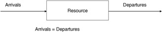
Figure 4.4: Resource in equilibrium.
The flow out of the resource is called its throughput. The mean service time is E[X], as defined previously, and the mean service rate is 1/E[X]. The utilization for this resource is defined as the fraction of time the resource is busy (U). The throughput of the resource must be equivalent to the service rate of the resource, when it is busy, times the fraction of the time it is busy.
This can be represented as:
| (4.22) |
If we have n identical devices in our system-for example, multiple CPUs with the same properties-then the throughput for these would be described as:
| (4.23) |
These simple relationships between utilization and expected time of service will be important measures in analyzing the performance of systems, as will be seen in later chapters.
Also of interest to the modeler is the size of the collection of jobs awaiting service at a resource and the time these jobs spend waiting for their service. First, we need to define the resource queue length. This is defined as the average number of jobs found waiting for service over the lifetime of this resource. Theoretically this can be found using the probability of having n waiting jobs times the number of jobs for all values of n:
| (4.24) |  |
where P(n) represents the probability that the resource's queue length is n. The mean queuing time (resource waiting time) can be found from:
| (4.25) |  |
where fq (q0) represents the probability density function for the resource's queuing times. From these observations it can be shown that:
| (4.26) |
This formula indicates that we can find the average queue length given that we know the average queuing time and the rate of arrivals λ (or serviced items) for the resource of interest. This simple observation was discovered by J. D. Little and is referred to as Little's Law. More will be said on this formula and its application to computer systems performance analysis in later chapters.
|
| < Free Open Study > |
|
EAN: 2147483647
Pages: 136