Chapter 4: General Measurement Principles

---

Overview

In modeling computer systems, we typically are interested in the service times of entities that utilize system resources. Entities in our discussion can represent a variety of operations on a computer system. For example, we may be interested in the time it takes to service an operating interrupt or, in a database system, the time to lock a data item in the database. The resources we are interested in are computer hardware elements and software resources. The entities represent the operations that are performed using the resources of the computer system. For example, if the resource is a central processing unit, a program operating on the CPU would have a service time composed of instruction execution (possibly driven by the instruction mix), memory management, I/O management, and secondary device access and transfer delays.

These components of the system under analysis are observable and possibly measurable. This does not mean that we need to measure all components precisely and completely as deterministic points in time. It may actually be more desirable to use average times and random service and arrivals to model these resources and programs. If the focus of review is the overall program operation, and not the components of this operation, then the service times will appear to be unpredictable and, therefore, can be assumed to be random. Without such assumptions, modeling a computer system would get bogged down in the extraction and determination of minute details, which may cloud our overall analysis.

Even though the service times for events may be unpredictable, we can still describe them in a way amenable to modeling and analysis with fairly good accuracy. For example, we can observe many event occurrences over a long period of time and deduce the composite average service time from this information with some degree of accuracy. Such approximations are sufficient for many models and for their analysis, as will be seen in later chapters.

One of the most important approximations concerning events and service distributions in a modeled system is that of probability distribution. It is important in modeled systems to have a measure of the possibility of some event occurring in relation to other events. The probability distribution looks to assign discrete probability values or continuous intervals of probable values to events. The assumption is that individual service times or events are independent and identically distributed (see Chapter 3). This is a reasonable approximation to reality under most conditions.

The simplest form of a probability distribution is found when we have a finite set of possible values. For example, the rolling of a fair die can only take on the values of {1,2,3,4,5,6} and no others. In addition, the probability of these individual values being rolled, given a fair die and an exhaustive number of trials, is 1/6 each. The possible values and a graphical representation are shown in Figure 4.1.

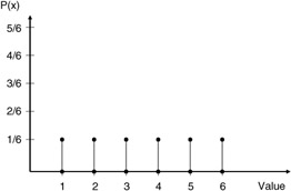
Figure 4.1: Probability distribution for a fair die.

In equation 4.1, P(x) represents the probability (or relative frequency) of value x occurring. In Chapter 5, we will see that P(x) must possess the properties that 0 ≤ P(x) ≤ 1 for all possible values of x from our set of possible values, and ∑ P(x) = 1.

When using such measures, the most important parameter when modeling is the mean or expected value. This value corresponds to the average value and is represented as:

(4.1) 

Given the distribution of equation 4.1, E[X] would be calculated as:

(4.2) 

An additional generalized measurement typically used is the nth moment and is computed as the sum of the x value raised to the nth power times the probability of this value of x occurrence, or:

(4.3) 

For our fair die example, the second moment would be found as:

(4.4)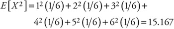 

A variation and more useful measure is the nth central moment, which is found by examining the difference between measured values and the expected value. The central moment is found by the formula:

(4.5) 

For our fair die example, the second central moment would be found as:

(4.6)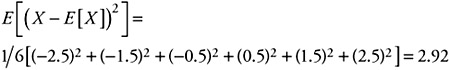 

This measure of the second central moment has another name: the variance. The variance can be refined to give us an important measure, called the standard deviation, by taking the square root of the variance. Typically the variance is written σ² . In our example, for the fair die, the standard deviation is found to be 1.7. The standard deviation tells us the average distance our measured values vary from the mean and can help in telling us how variable our data are. An additional measure concerning the relationship of actual values versus expected values is the coefficient of variation C_x. The coefficient of variation is defined as:

(4.7) 

In computer systems modeling it is possible to see coefficient of variation measures from below 1 to 10 and above. Most measures, however, will tend to fall somewhere between these values.

In modeling computer systems we often must characterize arrival rates and service rates using a variety of distribution functions. Typical distributions utilized include the exponential distribution, the normal distribution, the uniform distribution, and geometric distributions. We will mention them in overview in this chapter, discussing additional details in Chapter 5.

When looking at the values for an entity of interest, we have been examining how often the value occurs in comparison to all possible values. We have used the discrete probability distribution up to this point, since our examples assumed discrete values. Often in computer systems values for an entity of interest will not be discrete; they will be continuous. For example, the amount of time the CPU takes for every job it processes will typically consist of real values, not discrete values. Such measures require that the probability of a particular value we are interested in will vary over the full range of possible values. Such probability functions are continuous and are described by functions. The function describing the possible probability values for our entity of interest is called the probability density function (Figure 4.2), while the measure showing the systems probability is described by the probability distribution function (Figure 4.3). The probability density function gives us the actual value for the probability of some entity at a specific point in the state space for the item. The distribution function provides us with a probability measure indicating what the probability is that a value is less than or equal to a specific value.

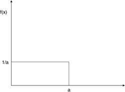
Figure 4.2: Probability density function.

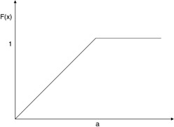
Figure 4.3: Probability distribution function.

For the measures we introduced for expected values, variance, and the central moment, the following changes in formula hold.

For the mean:

(4.8) 

for the variance:

(4.9)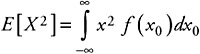 

and for the central moment:

(4.10)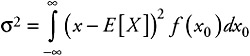 

For the distribution shown in Figure 4.2 the probability density function would be described as:

(4.11)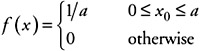 

and for the probability distribution function as:

(4.12)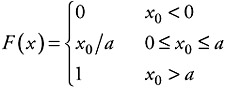 

The expected value for our example would be found as:

(4.13) 

The second moment for our example would be found as:

(4.14) 

and the variance called the central moment would be found as:

(4.15) 

One of the most important distributions for modeling computer systems is the exponential distribution (in particular the negative exponential). For the exponential distribution the probability density function is described as:

(4.16)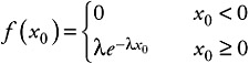 

and for the probability distribution function as:

(4.17)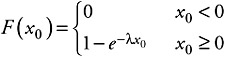 

The expected value for the exponential distribution is described as:

(4.18) 

The second moment is found as:

(4.19) 

The central moment is found as:

(4.20) 

and the coefficient of variation is found as:

(4.21) 

In later chapters we will see the importance of this distribution when examining computer systems. This distribution can be used in ways such that we can get very close approximations of general systems operations.

---