| Pivot tables are Excel's most powerful means of summarizing data. Whether you're interested in totaling expenses on a monthly basis, or finding the average income earned by people in various jobs, or getting a count of the number of items you've sold by product line, a pivot table is usually the way to do it in Excel. Because of their summary capabilities, pivot tables are tools not only for data analysis but also for data management. If you haven't yet used pivot tables extensively, you'll find this section a useful introduction. If you're an experienced user, you might prefer to skip ahead to the next section, "Preparing Data for Pivot Tables." Building a Pivot Table Figure 6.1 shows a simple example of a pivot table and its underlying data. Figure 6.1. Most pivot tables are based on either an Excel list or an external data source. 
It wouldn't be hard to build five array formulas that returned the total of units sold by region; for example =SUM(IF(B2:B39="South",D2:D39,0))
But why bother? The pivot table gives you those totals very quickly and easily. Here are the steps to take, given that you have an Excel list like the one shown in columns A through D of Figure 6.1. Be sure that you're using a list as described in Chapter 2, "Excel's Data Management Features," with column headers that name the fields. - Choose Data, PivotTable and PivotChart Report. Step 1 of the PivotTable Wizard shown in Figure 6.2 appears.
Figure 6.2. Basing a pivot table on another one means that they use the same data cache an efficient use of memory. 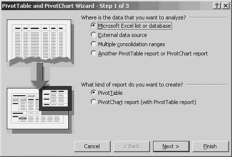
- In this instance, you would select Microsoft Excel List or Database, and PivotTable as a report type. (An Excel database is a legacy term for a list.) Choose Next.
- In step 2 of the PivotTable Wizard, shown in Figure 6.3, drag through the range of data in the worksheet so that its address, A1:D39 in Figure 6.1, appears in the Range box. Click Next.
Figure 6.3. If the underlying data is in a different workbook, you can click the Browse button to locate it. 
- Step 3 of the PivotTable Wizard appears (see Figure 6.4). Select the location for the pivot table and click Finish.
Figure 6.4. A pivot table by default starts in row 3 to leave room for a Page field. 
A schematic for the pivot table appears on the worksheet, along with the PivotTable Field List, as shown in Figure 6.5. To reproduce the pivot table shown in Figure 6.1, you would drag the Region field from the Field List into the Row Fields area, and drag the Units Sold field into the Data Items area. As soon as you put a field into the Data Items area, the pivot table replaces the schematic on the worksheet. Figure 6.5. If you prefer, you can use the Add To dropdown in the PivotTable Field List instead of dragging and dropping fields onto the worksheet. 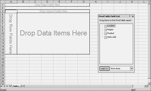
NOTE In Excel 97, the PivotTable Wizard is somewhat different from the one shown in Figures 6.2 through 6.5. In particular, there's a layout step in which you can design the pivot table. In subsequent versions, you create the layout directly on the worksheet as just described. You can get to the layout step by clicking the Layout button in the wizard's third step.
Reconfiguring a Pivot Table Why pivot table? Considering all that a pivot table is capable of, the reason for the term is relatively trivial. In Figure 6.1, if you click the button labeled Region, drag it into cell G3, and release the mouse button, the table pivots that is, the Row field Region becomes Column field Region. That's cute, but in nearly 10 years of using pivot tables to analyze and manage data, I've seldom had reason to pivot a table except to explain the term to people. Pivot tables are capable of much, much more than just pivoting. Figure 6.1 shows the Sum of Units Sold. Apart from Sum, there are many more summaries that you can choose, including Count, Average, Maximum, and Minimum. A numeric Data field defaults to Sum, and a text Data field defaults to Count. To select a different summary statistic, right-click any cell in the Data field, choose Field Settings from the shortcut menu, and locate the summary you want in the Summarize By list box. You can also have both a Row field and a Column field in a pivot table. This helps you assess the joint effect of the two fields. Figure 6.6 gives an example. Figure 6.6. To add Product as the Column field, drag it from the Field List to the Column area in the schematic shown in Figure 6.5. 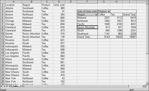
In addition, a pivot table can accommodate more than one Row field and Column field. Figure 6.7 shows the pivot table from Figure 6.6, but with an outer and an inner Row field and no Column field. To get two Row fields, for example, just drag them both into the schematic's Row area. Or, to revise the layout after the pivot table has been created, just drag the Region button directly to the right of the Product button. Figure 6.7. To get Region subtotals, right-click Region, choose Field Settings, choose Custom subtotals, and select a subtotal such as Sum. 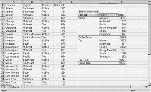
Besides Data, Row, and Column fields, pivot tables can also have Page fields. Page fields don't function in quite the same way as Row and Column fields. Their purpose is to enable you to select a subset of the underlying data and cause the pivot table to display only that subset. Figure 6.8 shows the data from Figure 6.1 using Product as a Page field, and displaying information for the Coffee product only. Figure 6.8. Your pivot table will include the records from each item in its Page field if you select All from its dropdown. 
If you want, you can use more than one Page field. If you do, they behave as though they were connected by Ands. For example, the pivot table shown in Figure 6.9 shows the Units Sold only for Coffee sales in the Northeast region. Figure 6.9. Only the locations in the Northeast region are shown when you choose that item in a Page field. 
You can set certain options in pivot tables. To do so, right-click a cell in the pivot table and choose Table Options from the shortcut menu. The dialog box shown in Figure 6.10 appears. Figure 6.10. Giving the pivot table a descriptive name is particularly helpful if you want to base another pivot table on it later. 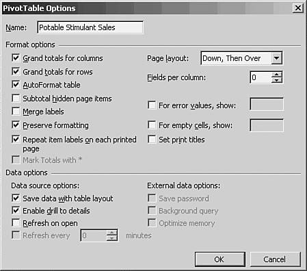
The more important of these options are as follows. Grand Totals for Columns, Grand Totals for Rows Refer to Figure 6.6, which shows a pivot table that includes both a Row field and a Column field. It shows Grand Totals in row 11 and in column I. If you clear the Grand Totals for Columns check box, the pivot table does not show the totals in row 11. If you clear the Grand Totals for Rows check box, the pivot table does not show the totals in column I. AutoFormat Table Excel offers 22 pivot table formats via the Format Report button on the PivotTable toolbar. If, having applied one of the formats, you want to remove the format from the pivot table, clear the AutoFormat Table check box. NOTE The format that's labeled None is not the same as the default format that's applied when you clear the AutoFormat Report check box.
Merge Labels Figure 6.7 shows a pivot table with an outer Row field, Product, and an inner Row field, Region. If you fill the Merge Labels check box, cells F5:F10 and cells F12:F17 are merged (as though you had chosen Format, Cells, Alignment and filled the Merge Cells check box). This also centers the labels in the merged cells both horizontally and vertically. Preserve Formatting When you're working with a pivot table's Data field, it's usually best to format it by right-clicking one of its cells, choosing Field Settings from the shortcut menu, and then clicking the Number button. That way, the number format you select is preserved if you pivot or refresh the table. But if you format the Data field's cells directly (or the cells in a Row or Column field) by selecting them and then choosing Cells from the Format menu, it's possible to lose the formatting (in particular, date formats). Filling the Preserve Formatting check box helps save direct cell formatting. Repeat Item Labels on Each Printed Page If you have a lengthy pivot table, it could span more than one printed page. And if you have only one Row field, the label that's in effect at the top of the second or subsequent printed page appears at the top of that page. But you might have more than one Row or Column field, as in Figure 6.7. In that case, the label of the outer Row or Column field is not repeated at the top of each page if this check box isn't filled. Page Layout Choose Down, Then Over to have multiple Page fields stacked vertically as in Figure 6.9, or choose Over, Then Down to have them appear side by side. Fields Per Column or Fields Per Row Depending on your choice for Page Layout, Page fields are either stacked in columns or side by side in rows. Suppose that you choose Down, Then Over. This option enables you to specify how many Page fields appear in a column before additional Page fields are placed in an adjacent column. If you choose Over, Then Down, you can specify how many page fields appear in a given row before additional ones are placed in the next row. For Error Values, Show If there are error values such as #DIV/0! or #REF! in the pivot table's data source, they appear in the pivot table itself. You might want a different value, such as Error, to appear in the pivot table. If so, fill this check box and type the value you want shown into the associated edit box. For Empty Cells, Show This check box and its associated edit box act in the same way as their counterparts do in For Error Values, Show, but for missing values instead of error values. Save Data with Table Layout A pivot table can store its underlying data in a cache. It's this cache that makes the pivot table so efficient at recalculating results when you pivot it or change it in some other way. If you clear this check box, the pivot table will not save a cache. When you re-open its workbook, you'll have to refresh the pivot table's data before you can change the table's structure. You do save some storage space by omitting the cache. Enable Drill to Details If you've saved the cache along with the pivot table, you can get at the underlying data for any cell in the Data field. Just double-click that cell, and Excel inserts a new worksheet with a list. The list contains all the fields for all the records that belong to the cell you double-clicked. If you clear this check box, you won't be able to do that, and you might want to prevent other users of your pivot table from seeing detail records. If you want to be able to drill to details, you must also have filled the Save Data with Table Layout check box. Refresh on Open This is a very useful option if the data that forms the basis for the pivot table changes from time to time. If the check box is filled, the pivot table automatically refreshes itself from the data source when you open the workbook. TIP Many of the workbooks I prepare for my clients have as many as 20 pivot tables that are based on external data sources such as Access databases. It can take a frustratingly long time for all the pivot tables in those workbooks to refresh. In such cases, I prefer to deselect this option and use the workbook's Open event to run VBA code that asks the user if he wants to refresh the pivot tables. If he does, the event runs more VBA code that refreshes all the pivot tables in the workbook.
The following options are available only if the pivot table is based on an external data source. Refresh Every x Minutes You can cause the pivot table to refresh itself from the data source by filling the check box and setting the number of minutes with the spinner. Save Password If the external data source is password-protected, you can cause Excel to save the password so that you (and other users of the workbook) won't have to supply it when the pivot table is refreshed later on. This is a more secure way of saving the data source's password than to save it with a DSN file, which can be read with something as ubiquitous and basic as Notepad. Background Query If your external data source supports asynchronous queries, you might want to use this option. If the check box is filled, you can continue doing other work in Excel as the query refreshes the pivot table. If the check box is cleared, you'll have to wait until the refresh is complete before you can do anything else in the workbook. This option is useful mainly in very slow networked environments. Optimize Memory If you fill this check box, Excel takes some preliminary steps before it refreshes a pivot table. In particular, Excel determines how many unique items there are in the pivot table's row and column fields. By doing so, it's able to manage its memory allocations more efficiently. You might notice a slight drop-off in performance as Excel makes these checks. |