| The OFFSET function returns a reference to a cell, or to a range of cells, and it displays their contents. Figure 2.2 has a basic example of OFFSET. Figure 2.2. OFFSET is one good way to rearrange data from a table. 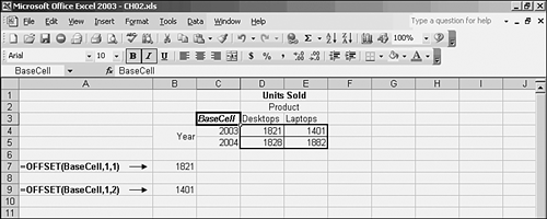
Understanding the Basis Cell OFFSET needs a cell reference to use as a basis. You will also tell OFFSET how many rows and how many columns to shift, or offset, but first it needs to know which cell to shift from. The whole idea behind the OFFSET function is that you want the address of a range of cells that are near to some other cell. For example, you might want to use the address of the range of cells in a table so that you can get their sum, but you don't want to include the row of labels at the top of the table. You could use the cell in the table's upper-left corner as the basis cell to tell OFFSET where to start. In Figure 2.2, OFFSET uses a cell named BaseCell as its basis. For example, the formula with the OFFSET function, as used in cell B9, is =OFFSET(BaseCell,1,2)
So, cell B9 uses the OFFSET function to Start with the cell named BaseCell, which is cell $C$3. OFFSET's second argument tells it how many rows to shift. In this case, the second argument is 1, so OFFSET shifts down one row below BaseCell, into row 4. OFFSET'S third argument tells it how many columns to shift. In this case, the third argument is 2, so OFFSET shifts two columns to the right from BaseCell, into column E.
In other words, cell B9 displays the contents of the cell that is one row below and two columns right of BaseCell. That is cell E4, and its value, 1401, is the one you see in B9. Array-Entering OFFSET to Return Several Cells OFFSET has two other arguments: Height and Width. These refer to the height of the range in rows, and the width of the range in columns, that you want OFFSET to return. (They need to be positive numbers: Excel doesn't know how to interpret a range that's 2 rows high.) So, this formula =OFFSET(BaseCell,1,1,2,2)
would return a range that's offset from BaseCell by one row and one column, and that is two rows high and two columns wide, as shown in Figure 2.3. Figure 2.3. The curly brackets around the formula tell you that it's an array formula. 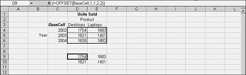
Typically, OFFSET is used to return just some of the rows or some of the columns in a source range. It can also be used to return, say, a 3 by 3 section of a 7 by 7 source range. TIP OFFSET's Height and Width arguments are particularly powerful when used to return successively larger square sections of an array of values, as is often required in quantitative analysis. For example =OFFSET(A1,0,0,2,2) =OFFSET(A1,0,0,3,3) =OFFSET(A1,0,0,4,4)
But notice in Figure 2.3 that there are curly brackets, sometimes termed French braces, around the formula. This means that it is not a regular Excel formula, but an array formula. Array formulas often, but not always, occupy a range of multiple cells. They usually take arrays as one or more arguments. Array formulas were mentioned (without much explanation) in the first section of this chapter. You enter an array formula with a special key combination: Ctrl+Shift+Enter. In words, you hold down the Ctrl and Shift keys simultaneously, and press Enter. Your formula appears in the formula bar surrounded by curly braces, just as shown in Figure 2.3. CAUTION Don't type the curly braces yourself. If you do, Excel will interpret the formula as text.
You find array formulas in many Excel worksheets that have intermediate to advanced uses. In fact, several Excel functions require that you array-enter them or they won't work as intended; among them are MMULT, MDETERM, LINEST, LOGEST, and FREQUENCY. Also keep in mind that you need to select the range that the formula will occupy before you begin to enter it. Of course, this requires that you know the dimensions of the array that the function will return. To array-enter the OFFSET function shown in Figure 2.3, follow these three steps in this specific order: - Using Insert, Name, Define, name cell $C$3 BaseCell.
- Select the range D9:E10.
- Click in the Formula Bar, and type this: =OFFSET(BaseCell,1,1,2,2).
- Hold down Ctrl and Shift, and press Enter.
This array-entered formula, with the help of the OFFSET function, returns a reference to D4:E5--the range that is offset from the basis cell C3 by one row and one column, and that is two rows high and two columns wide. If instead you had array-entered this formula =OFFSET(BaseCell,1,1,2,3)
it would have returned a range two rows high and three columns wide. But you would have had to begin by selecting a 2 row by 3 column range before array-entering the formula. |