Creating a Basic PivotTable
3 4
Once you have constructed a query containing suitable fields, you can create a new form by using the PivotTable Wizard or by selecting AutoForm: PivotTable in the New Form dialog box. Unlike most other Access wizards, the PivotTable Wizard isn’t all that helpful. Basically, the wizard lets you select a data source and (if you want) select fields from the data source.
Switching to PivotTable or PivotChart View in an Existing Access Form
The simplest way to create a PivotTable or PivotChart in Access is to switch to PivotTable view or PivotChart view for an existing Access form. You can do this by choosing View, PivotTable or View, PivotChart, or by selecting PivotTable or PivotChart on the View selector on the Form toolbar.
If the PivotTable or PivotChart view is unavailable, you can open the form’s properties sheet and set the Allow PivotTable View or Allow PivotChart View property to Yes. Keep in mind, however, that this property might have been set to No because the form’s record source isn’t suitable for a PivotTable or PivotChart. In that case, you might need to create a new form to get a useful PivotTable or PivotChart view.
After you switch to PivotTable or PivotChart view, a blank PivotTable or PivotChart layout will appear, with drop zones for dragging row fields, column fields, and filter fields.
After you complete the two wizard pages, you end up with a blank PivotTable and the PivotTable field list, identical to what appears when you switch to PivotTable view for a form or select AutoForm: PivotTable in the New Form dialog box (as described later in this section). Because the PivotTable Wizard doesn’t provide any extra help, it’s faster to use one of the other techniques for creating a PivotTable.
note
When I use the term PivotTable form, I don’t mean a special type of database object. A PivotTable form is just a standard Access form, but one designed from the start to produce a useful PivotTable view—which isn’t always the case if you switch to PivotTable view from an existing form. Forms are often based on a single table, whereas a PivotTable generally needs data from several linked tables.
To conveniently create a PivotTable form, follow these steps:
- Prepare a query with all (and only) the fields you want to work with in the PivotTable.
- In the Forms group of the Database window, click the New button, or choose Insert, Form.
- Select AutoForm: PivotTable from the list.
- In the New Form dialog box, select the prepared query to use as the PivotTable form’s data source from the drop-down list, as shown in Figure 12-4, and then click OK.
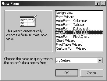
Figure 12-4. Select AutoForm: PivotTable and a query to create a new PivotTable form.
- A form based on the selected query opens in PivotTable view, as shown in Figure 12-5, with the PivotTable field list visible so that you can select fields for the PivotTable to display.
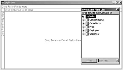
Figure 12-5. A new PivotTable form with the PivotTable field list for selecting fields.
InsideOut
You can’t directly create a PivotTable report, but you can create a form set up for PivotTable view and then save it as a report. The result is not a true PivotTable, however—it’s just an image of one (meaning that it’s not interactive). This image is basically the same as printing the PivotTable from a form.
Choosing Fields for the PivotTable
The next step is to select the fields to use for row headings, column headings, and data. The PivotTable field list provides a list of all the fields in the form’s record source. If you prepared a query in advance, you’ll see just a few appropriate fields. (This is one of the advantages of preparing a query for a PivotTable.) Otherwise, you’ll see a long list of all the fields in the data source, only a few of which are appropriate for use in a PivotTable.
InsideOut
Lookup fields (such as Customer ID) are listed in the PivotTable field list under the names of the linked fields in the other tables. (For example, Customer ID might be listed as the Customer Name field.) However, when you drag a lookup field to the PivotTable, you’ll see the Customer ID field on the grid, not the Customer Name field, which probably isn’t what you want, since most likely users will want to see customer names on the PivotTable, not just Customer IDs. (The Customer Name is far more meaningful to a human than the numeric Customer ID field.) To prevent such problems, create a query containing the fields you want to use from each table. Don’t rely on picking up a field from another table by using a lookup field.
You need to drag one or more fields to the Row Fields drop zone, another field to the Column Fields drop zone, and a third field to the Totals Or Detail Fields drop zone. (We’ll ignore the Filter Fields drop zone for now; its use is optional. You’ll learn more about using the Filter Fields drop zone later in this section.)
tip
As an alternative to dragging a field from the PivotTable field list to a drop zone, you can select the field and then select the drop zone from the Add To drop-down list at the bottom of the PivotTable field list.
For example, to drag fields to a PivotTable to display data for a text field (CompanyName) in rows, with columns arranging data by months, follow these steps:

In this example, we’ll use fields from the sample qryOrders query in the Test Access 2002 sample database on the companion CD, but the same general principles apply to any data source used to provide fields for a PivotTable.
- Drag a text field containing data you want to see in rows (in this case, CompanyName) from the PivotTable field list to the Row Fields drop zone on the PivotTable, as shown in Figure 12-6.
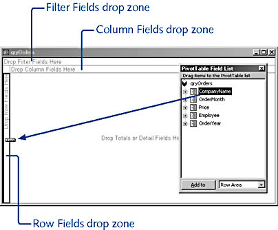
Figure 12-6. Drag a field from the field list to the Row Fields drop zone to use its data for rows in the PivotTable.
tip
If the PivotTable field list isn’t visible, right-click the PivotTable and choose Field List from the shortcut menu, or press the F8 hot key.The company names appear along the left side of the PivotTable.
note
The drop zone border turns bright blue when the dragged field is positioned correctly for dropping. Fields that have been dragged to the PivotTable appear in boldface in the field list. - Drag the text field containing data you want to see in columns (in this case, OrderMonth) from the PivotTable field list to the Column Fields drop zone.
Month columns will appear along the top of the PivotTable, as shown in Figure 12-7.
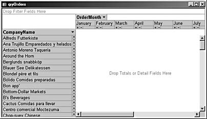
Figure 12-7. The PivotTable now has row and column headings.
- Drag the field containing data for the PivotTable (in this case, Price) to the Totals Or Detail Fields drop zone. The detail prices appear in the center of the form, in the appropriate rows and columns, as shown in Figure 12-8.
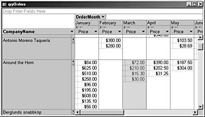
Figure 12-8. Price data now appears in the Detail area of the PivotTable.
- If you want to filter your PivotTable data, you can drag a field to the Filter Fields drop zone. For example, if you want to see only orders for a specific year, drag the OrderYear field to the Filter Fields drop zone, clear the check boxes for the years you want to exclude on the drop-down list, and then click OK, as shown in Figure 12-9.
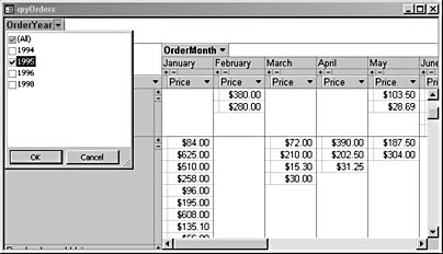
Figure 12-9. Set up a filter condition by deselecting years in the OrderYear drop-down list.
tip
You also clear the All check box at the top of the list, and then check the items you want to include in the filter condition. - To sum the prices for each row/column combination, click the Price selector over one of the columns (the prices will turn blue to indicate that they’re selected), click the AutoCalc button on the PivotTable toolbar, and choose Sum from the drop-down menu, as shown in Figure 12-10.
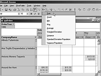
Figure 12-10. Choose Sum from the AutoCalc menu to create a column subtotal for each row of data.
Price subtotals will appear for each row/column combination, as shown in Figure 12-11.
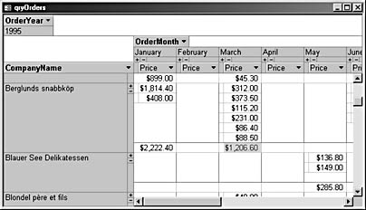
Figure 12-11. The PivotTable now shows a monthly subtotal for each row of data.
- To show or hide the details for a row, click the tiny plus and minus buttons to the right of the company name in each row. (Click the Hide Details and Show Details buttons on the PivotTable toolbar to hide or show details for the entire PivotTable.)
- To display more than one summary function, click AutoCalc again and select another function. When details are hidden, the summary type is listed under the top row of column headings (in this case, months). A ScreenTip provides information about a particular summary value when you hover your mouse pointer over it, as illustrated in Figure 12-12, which shows both Sum and Count summaries of prices.
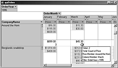
Figure 12-12. A PivotTable shows details of the Sum and Count summaries of Price in a ScreenTip.
tip
To remove a summary row from a PivotTable, right-click the summary value, and choose Remove from the shortcut menu. - Scroll to the bottom right of the PivotTable to see a Grand Total row and a Grand Total column.
note
PivotTables and PivotCharts are actually Excel objects embedded in Access objects. If you use the PivotTable Wizard or choose the AutoForm: PivotTable selection in the New Form dialog box to create a PivotTable form, an Excel PivotTable object is embedded in an Access form. This might explain why some of the tools on the PivotTable toolbar are similar to Excel tools. However, if you look at PivotTables in Excel 2002, you’ll see that they appear rather different from Access 2002 PivotTables.
Fine-Tuning PivotTables with Advanced Tools
You now have a useful PivotTable, but there are several additional ways you can modify it, if needed. You can make stylistic changes by specifying the font, color, and size of the PivotTable components; add captions to explain portions of the PivotTable; and perform advanced filtering and grouping. In this section, we’ll look at these and other advanced tools for working with PivotTables.
Filtering PivotTable Data
To filter data by a value in a field, follow these steps:
- Click the arrow to the right of the field name you want to use for filtering.
- Select one or more values from the drop-down list.
- Click OK.
In our example PivotTable, which is filtered by year using a filter field, you can also filter on the CompanyName field by clicking the CompanyName drop-down arrow and selecting a particular company to filter by, as shown in Figure 12-13.
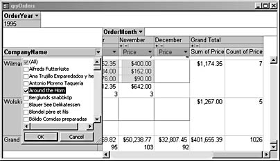
Figure 12-13. You can select a specific company name to filter PivotTable data for just that company.
The filtered PivotTable now contains data for only the company you specified.
Setting PivotTable Properties
In addition to using the PivotTable toolbar buttons to work with PivotTables, you can also click the Properties button to open the PivotTable properties sheet, which contains several tabs, where you can set more options for the PivotTable.
note
The PivotTable properties sheet contains a different selection of tabs depending on what element of the PivotTable is selected when the properties sheet is opened.
Formatting a PivotTable On the Format tab of the properties sheet, you can set a number of standard formatting options for the selected PivotTable element, including font, size, and color. To do so, follow these steps:
- Right-click the element in the PivotTable you want to modify, and choose Properties from the shortcut menu.
- Click the Format tab, and change the desired options.
- Close the properties sheet.
For example, to make subtotals bold and bright blue, right-click any subtotal in the PivotTable, open the PivotTable properties sheet, and select the Format tab. Click the Bold button, and then click the down arrow to the right of the Font Color button to open a drop-down list, shown in Figure 12-14, where you can specify the exact shade of blue you want.
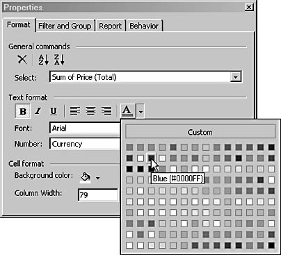
Figure 12-14. You can format PivotTable components using settings on the Format tab of the PivotTable properties sheet.
Modifying PivotTable captions The Captions tab lets you modify the appearance of the row, column, and filter captions (the text that describes the Row, Column, and Filter fields) in the PivotTable. To do so, follow these steps:
- Right-click the row, column, or filter caption in the PivotTable you want to modify, and choose Properties from the shortcut menu.
- Click the Captions tab, and change the desired options.
- Close the properties sheet.
For example, if your field names don’t contain spaces (like the CompanyName field in the example) and you want to add spaces to make them more legible, you could select a field and add spaces to its caption, as shown in Figure 12-15.
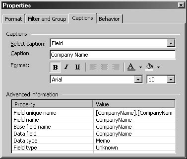
Figure 12-15. You can modify a PivotTable’s captions on the Captions tab of the PivotTable properties sheet.
Using advanced filtering and grouping techniques The Filter And Group tab provides more advanced options for filtering and grouping a PivotTable. You can make a PivotTable display the specified number of items at the top or bottom of a list, based on count or percentage, or group items by prefix characters (somewhat like an Access reportgrouped by the first letter—see Chapter 7, "Using Reports to Print Data"). To do so, follow these steps:
- Right-click the filter or grouping element in the PivotTable you want to modify, and choose Properties from the shortcut menu.
- Click the Filter And Group tab, and change the desired options.
- Close the properties sheet.
Figure 12-16 shows the settings for filtering a PivotTable by the top 10 percent of data.
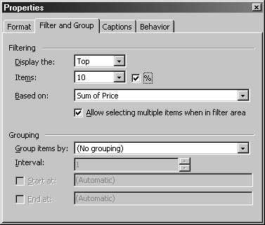
Figure 12-16. You can filter a PivotTable for the top 10 percent of data values using the Filter And Group tab.
Modifying how data is displayed in a PivotTable The Report tab of the PivotTable properties sheet allows you to set generic PivotTable options, such as whether the PivotTable should display empty rows and columns. To do so, follow these steps:
- Right-click an element in the PivotTable you want to modify, and choose Properties from the shortcut menu.
- Click the Report tab, and change the desired options.
- Close the properties sheet.
For instance, choosing the Row Headings option on the Report tab displays the label Sum of Price next to the row headings in the example PivotTable, as shown in Figure 12-17. Several other options on this tab let you specify whether empty rows and columns, calculated items, or ScreenTips will be displayed in the PivotTable.
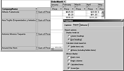
Figure 12-17. You can change how totals are displayed by configuring settings on the Report tab of the PivotTable properties sheet.
The Behavior tab, shown in Figure 12-18, lets you modify some more intricate details of the appearance of the PivotTable, such as whether the Expand indicators are displayed in the PivotTable.
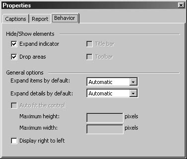
Figure 12-18. You can modify some interactive elements of a PivotTable on the Behavior tab of the properties sheet.
InsideOut
There’s no Undo command for PivotTables (unlike for forms, reports, and other Access database objects, which have an Undo button on the toolbar), so if you make amistake, you have to manually replace or modify the incorrect element. Hopefully, Undo for PivotTables will be added in the next version of Access.
Pivoting a PivotTable
Unlike crosstab queries, PivotTables (as their name implies) can be pivoted—that is, you can swap the vertical and horizontal data simply by dragging the fields to opposite locations. For example, to view the company names in our sample PivotTable as column headings and the months as row headings, all you have to do is drag the CompanyName field to the Column Fields drop zone and the Years field to the Row Fields drop zone. The Months field will accompany the Years field as the new row fields, with Years as the outer field and Months as the inner field. The resulting PivotTable is shown in Figure 12-19.
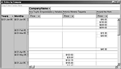
Figure 12-19. A PivotTable lets you swap row and column headings simply by dragging fields.
This flexibility gives PivotTables a great advantage over crosstab queries, as users can manipulate the rows and columns, filter the data, and add subtotals in PivotTable view to analyze data as they prefer.
EAN: 2147483647
Pages: 172