9.1 The Circuit-Diagnosis Problem

9.1 The Circuit-Diagnosis Problem

The circuit-diagnosis problem provides a good test bed for understanding the issues involved in belief revision. A circuit consists of a number of components (AND, OR, NOT, and XOR gates) and lines. For example, the circuit of Figure 9.1 contains five components, X₁, X₂, A₁, A₂, O₁ and eight lines, l₁, …, l₈. Inputs (which are either 0 or 1) come in along lines l₁, l₂, and l₃. A₁ and A₂ are AND gates; the output of an AND gate is 1 if both of its inputs are 1, otherwise it is 0. O₁ is an OR gate; its output is 1 if either of its inputs is 1, otherwise it is 0. Finally, X₁ and X₂ are XOR gates; the output of a XOR gate is 1 iff exactly one of its inputs is 1.

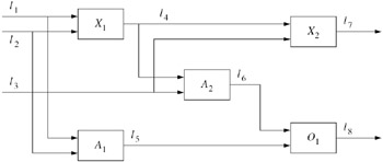
Figure 9.1: A typical circuit.

The circuit-diagnosis problem involves identifying which components in a circuit are faulty. An agent is given a circuit diagram as in Figure 9.1; she can set the values of input lines of the circuit and observe the output values. By comparing the actual output values with the expected output values, the agent can attempt to locate faulty components.

The agent's knowledge about a circuit can be modeled using an epistemic structure M_diag^K = (W_diag, _diag, π_diag). Each possible world w ∈ W_diag is composed of two parts: fault(w), the failure set, that is, the set of faulty components in w, and value(w), the value of all the lines in the circuit. Formally, value(w) is a set of pairs of the form (l, i), where l is a line in the circuit and i is either 0 or 1. Components that are not in the failure sets perform as expected. Thus, for the circuit in Figure 9.1, if w ∈ W_diag and A₁ ∉ fault(w), then (l₅, 1) is in value(w) iff both (l₁, 1) and (l₂, 1) are in value(w). Faulty components may act in arbitrary ways (and are not necessarily required to exhibit faulty behavior on all inputs, or to always act the same way when given the same inputs).

What language should be used to reason about faults in circuits? Since an agent needs to be able to reason about which components are faulty and the values of various lines, it seems reasonable to take

where faulty(c_i) denotes that component c_i is faulty and hi(l_i) denotes that line l_i in a "high" state (i.e., has value 1). Define the interpretation π_diag in the obvious way:

π_diag(w)(faulty(c_i)) = true if c_i ∈ fault(w), and π_diag(w)(hi(l_i)) = true if (l_i, 1) ∈ value(w).

The agent knows which tests she has performed and the results that she observed. Let obs(w) ⊆ value(w) consist of the values of those lines that the agent sets or observes. (For the purposes of this discussion, I assume that the agent sets the value of a line only once.) I assume that the agent's local state consists of her observations, so that (w, w′) ∈ _diag if obs(w) = obs(w′). For example, suppose that the agent observes hi(l₁) ∧ hi(l₂) ∧ hi(l₃) ∧ hi(l₇) ∧ hi(l₈). The agent then considers possible all worlds where lines l₁, l₂, l₃, l₇ and l₈ have value 1. Since these observations are consistent with the circuit being correct, one of these worlds has an empty failure set. However, other worlds are possible. For example, it might be that the AND gate A₂ is faulty. This would not affect the outputs in this case, since if A₁ is nonfaulty, then its output is "high", and thus, O₁'s output is "high" regardless of A₂'s output.

Now suppose that the agent observes hi(l₁) ∧ hi(l₂) ∧ hi(l₃) ∧ hi(l₇) ∧ hi(l₈). These observations imply that the circuit is faulty. (If l₁ and l₃ are "high" and l₂ is "low", then the correct values for l₇ and l₈ should be "low" and "high", respectively.) In this case there are several failure sets consistent with the observations, including {X₁}, {X₂, O₁}, and {X₂, A₂}.

In general, there is more than one explanation for the observed faulty behavior. Thus, the agent cannot know exactly which components are faulty, but she may have beliefs on that score. The beliefs depend on her plausibility measure on runs. One way of constructing a reasonable family of plausibility measures on runs is to start with a plausibility measure over possible failures of the circuit. I actually construct two plausibility measures over failures, each capturing slightly different assumptions. Both plausibility measures embody the assumptions that (1) failures are unlikely and (2) failures of individual components are independent of one another. It follows that the failure of two components is much more unlikely than the failure of any one of them. The plausibility measures differ in what they assume about the relative likelihood of the failure of different components.

The first plausibility measure embodies the assumption that the likelihood of each component failing is the same. This leads to an obvious order of failure sets: if f₁ and f₂ are two failure sets, then f₁ ≽₁ f₂ if (and only if) |f₁|≤|f₂|, that is, if f₁ consists of fewer faulty components than f₂. The order on failure sets, in turn, leads to a total order on worlds: w₁ ≽₁ w₂ iff fault(w₁) ≽₁ fault(w₂). Using the construction of Section 2.7, this ordering on worlds can be lifted to a total order ≽^s₁ on sets of sets of worlds. Moreover, by Theorem 2.7.5 and Exercise 2.49, ≻^s₁ can be viewed as a qualitative plausibility measure. Call this plausibility measure Pl₁.

Pl₁ can also be constructed by using probability sequences. Let μ_m be the probability measure that takes the probability of a component failing to be 1/m and takes component failures to be independent. Then for a circuit with n components,

It is now easy to check that Pl₁ is just the plausibility measure obtained from the probability sequence (μ₁, μ₂, μ₃, …) using the construction preceding Theorem 8.4.12 (Exercise 9.1(a)). Note that the probability of a component being faulty tends to 0 as the subscript increases. However, at each measure in the sequence, each component is equally likely to fail and the failures are independent.

In some situations it might be unreasonable to assume that all components have equal failure probability. Moreover, the relative probability of failure for various components might be unknown. Without assumptions on failure probabilities, it is not possible to compare failure sets unless one is a subset of the other. This intuition leads to a different order on failure sets. Define f ≽₂ f′ iff f ⊆ f′. Again this leads to an ordering on worlds by taking w₁ ≽₂ w₂ iff fault(w₁) ≽₂ fault(w₂) and, again, ≽^s₂ determines a plausibility measure Pl₂ on W_diag. It is not hard to find a probability sequence that gives the same plausibility measure (Exercise 9.1(b)).

Pl₁ and Pl₂ determine structures M₁ and M₂, respectively, for knowledge and plausibility: M_i = (W_diag, _diag, _diag,i, π_diag), where _diag,i(w) = (_diag(w), P1ⁱ_w) and P1ⁱ_w(U) = P1_i(_diag(w) ∩ U), for i = 1, 2.

Suppose that the agent makes some observations o. In both M₁ and M₂, if there is a world w compatible with the observations o and fault(w) = ∅, then the agent believes that the circuit is fault-free. That is, the agent believes the circuit is faultfree as long as her observations are compatible with this hypothesis. If not, then the agent looks for a minimal explanation of her observations, where the notion of minimality differs in the two structures. More precisely, if f is a failure set, let Diag(f) be the formula that says that exactly the failures in f occur, so that (M, w) ⊨ Diag(f) if and only if fault(w) = f. For example, if f ={c₁, c₂}, then Diag(f) = faulty(c₁) ∧ faulty(c₂) ∧ faulty(c₃) ∧ … ∧ faulty(c_n). The agent believes that f is a possible diagnosis (i.e., an explanation of her observations) in world w of structure M_i if (M_i, w) ⊨ B Diag(f). The set of diagnoses the agent considers possible is DIAG(M, w) ={f : (M, w) ⊨ B Diag(f)}. A failure set f is consistent with an observation o if it is possible to observe o when f occurs, that is, if there is a world w in W such that fault(w) = f and obs(w) = o.

Proposition 9.1.1

1. DIAG(M₁, w) contains all failure sets f that are consistent with obs(w) such that there is no failure set f′ with |f′| < |f| that is consistent with obs(w).

2. DIAG(M₂, w) contains all failure sets f that are consistent with obs(w) such that there is no failure set f′ with f′ ⊂ f that is consistent with obs(w). (Recall that ⊂ denotes strict subset.)

Proof See Exercise 9.2.

Thus, both DIAG(M₁, w) and DIAG(M₂, w) consist of minimal sets of failure sets consistent with obs(w), but for different notions of minimality. In the case of M₁, "minimality" means "of minimal cardinality", while in the case of M₂, it means "minimal in terms of set containment." More concretely, in the circuit of Figure 9.1, if the agent observes hi(l₁) ∧ hi(l₂) ∧ hi(l₃) ∧ hi(l₇) ∧ hi(l₈), then in M₁ she would believe that X₁ is faulty, since {X₁} is the only diagnosis with cardinality one. On the other hand, in M₂ she would believe that one of the three minimal diagnoses occurred: {X₁}, {X₂, O₁}, or {X₂, A₂}.

The structures M_i, i = 1, 2, model a static situation. They describe the agent's beliefs given some observations, but do not describe the process of belief revision—how those beliefs change in the light of new observations. One way to model the process is to add time to the picture and model the agent and the circuit as part of an interpreted plausibility system. This can be done using a straightforward modification of what was done in the static case.

The first step is to describe the agent's set of local states and the set of environment states. In the spirit of the static model, I assume that the agent sets the value of some lines in the circuit and observes the value of others. Let o_{(r, m)} be a description of what the agent has set/observed in round m of run r, where o_{(r, m)} is a conjunction of formulas of the form hi(l_j) and their negations. The form of the agent's local states depends on the answers to some of the same questions that arose in the Listener-Teller protocol of Section 6.7.1. Does the agent remember her observations? If not, what does she remember of them? For simplicity here, I assume that the agent remembers all her observations and makes an additional observation at each round. Given these assumptions, it seems reasonable to model the agent's local state at a point (r, m) as the sequence 〈o_{(r, 1)}, …, o_{(r, m)}〉. Thus, the agent's initial state at (r, 0) is 〈〉, since she has not made any observations; after each round in r, a new observation is added.

The environment states play the role of the worlds in the static models; they describe the faulty components of the circuit and the values of all the lines. Thus, I assume that the environment's state at (r, m) is a pair (fault(r, m), value(r, m)), where fault(r, m) describes the failure set at the point (r, m) and value(r, m) describes the values of the lines at (r, m). Of course, o_{(r, m)} must be compatible with value(r, m): the values of the lines that the agent observes/sets at (r, m) must be the actual values. (Intuitively, this says that the agents observations are correct and when the agent sets a line's value, it actually has that value.) Moreover, fault(r, m) must be compatible with value(r, m), in the sense discussed earlier: if a component c is not in fault(r, m), then it outputs values according to its specification, while if c is in fault(r, m), then it exhibits its faultiness by not obeying its specification for all inputs. I further assume that the set of faulty components does not change over time; this is captured by assuming fault(r, m) = fault(r, 0) for all r and m. On the other hand, I do not assume that the values on the lines are constant over time since, by assumption, the agent can set certain values. Let _diag consist of all runs r satisfying these requirements.

There are obvious analogues to Pl₁ and Pl₂ defined on runs; I abuse notation and continue to call these Pl₁ and Pl₂. For example, to get Pl₁, first define a total order ≽₁ on the runs in _diag by taking r₁ ≽₁ r₂ iff fault(r₁, 0)) ≽₁ fault(r₂, 0); then ≽^s₁ gives a total order on sets of runs, which can be viewed as a plausibility measure on runs. Similarly, the plausibility measure Pl₂ on _diag is the obvious analogue to Pl₂ defined earlier on w_diag.

Pl₁ and Pl₂ determine two interpreted plausibility systems whose set of runs in _diag; call them 퓙₁ and 퓙₂. Since Pl₁ and Pl₂ put plausibility on all of _diag, 퓙₁ and 퓙₂ are actually SDP systems (see Section 6.4). In each system, the agent believes that the failure set is one of the ones that provides a minimal explanation for her observations, where the notion of minimal depends on the plausibility measure. As the agent performs more tests, her knowledge increases and her beliefs might change.

Let DIAG(퓙, r, m) be the set of failure sets (i.e., diagnoses) that the agent considers possible at the point (r, m) in the system 퓙. Belief change in 퓙₁ is characterized by the following proposition, similar in spirit to Proposition 9.1.1:

Proposition 9.1.2

If there is some f ∈ DIAG(퓙₁, r, m) that is consistent with the new observation o_{(r, m+1)}, then DIAG(퓙₁, r, m + 1) consists of all the failure sets in DIAG(퓙₁, r, m) that are consistent with o_{(r, m+1)}. If all f ∈ Bel(퓙₁, r, m) are inconsistent with o_{(r, m+1)}, then Bel(퓙₁, r, m + 1) consists of all failure sets of cardinality j that are consistent with o_{(r, m+1)}, where j is the least cardinality for which there is at least one failure set consistent with o_{(r, m+1)}.

Proof See Exercise 9.3.

Thus, in 퓙₁, if an observation is consistent with the pre-observation set of most likely explanations, then the post-observation set of most likely explanations is a subset of the pre-observation set of most likely explanations (the subset consisting of those explanations that are consistent with the new observation). On the other hand, a surprising observation (one inconsistent with the current set of most likely explanations) has a rather drastic effect. It easily follows from Proposition 9.1.2 that if o_{(r, m+1)} is surprising, then DIAG(퓙₁, r, m) ∩ DIAG(퓙₁, r, m + 1) = , so the agent discards all her pre-observation explanations. Moreover, an easy induction on m shows that if DIAG(퓙₁, r, m) ∩ DIAG(퓙₁, r, m + 1) = , then the cardinality of the failure sets in DIAG(퓙₁, r, m + 1) is greater than the cardinality of the failure sets in DIAG(퓙₁, r, m). Thus, in this case, the explanations in DIAG(퓙₁, r, m + 1) are more "complicated" than those in Bel(퓙₁, r, m), in the sense that they involve more failures.

Belief change in 퓙₂ is quite different, as the following proposition shows. Roughly speaking, it says that after making an observation, the agent believes possible all minimal extensions of the diagnoses she believed possible before making the observation.

Proposition 9.1.3

DIAG(퓙₂, r, m + 1) consists of the minimal (according to ⊆) failure sets in {f′ : f′ ⊇ f for some f ∈ DIAG(퓙₂, r, m)} that are consistent with o_{(r, m+1)}.

Proof See Exercise 9.4.

As with 퓙₁, diagnoses that are consistent with the new observation are retained. However, unlike 퓙₁, diagnoses that are discarded are replaced by more complicated diagnoses even if some of the diagnoses considered at (r, m) are consistent with the new observation. Moreover, while new diagnoses in DIAG(퓙₁, r, m + 1) can be unrelated to the diagnoses in DIAG(퓙₁, r, m), in 퓙₂ the new diagnoses must be extensions of some discarded diagnoses. Thus, in 퓙₁ the agent does not consider new diagnoses as long as the observation is not surprising. On the other hand, in 퓙₂ the agent has to examine new candidates after each test.

This point is perhaps best understood by example.

Example 9.1.4

Suppose that in the circuit of Figure 9.1, the agent initially sets l₁ = 1 and l₂ = l₃ = 0. If there were no failures, then l₄ and l₇ would be 1, while, l₅, l₆, and l₈ would be 0. But if the agent observes that l₈ is 1, then in both systems the agent would believe that exactly one of X₁, A₁, A₂, or O₁ was faulty; that would be the minimal explanation of the problem, under both notions of minimality. Now suppose that the agent later observes that l₇ = 0 while all the other settings remain the same. In that case, the only possible diagnosis according to Pl₁ is that X₁ is faulty. This is also a possible diagnosis according to Pl₂, but there are three others, formed by taking X₂ and one of A₁, A₂, or O₁. Thus, even though a diagnosis considered possible after the first observation—that X₁ is faulty—is consistent with the second observation, some new diagnoses (all extensions of the diagnoses considered after the first observation) are also considered.