Applying Conditional Formatting

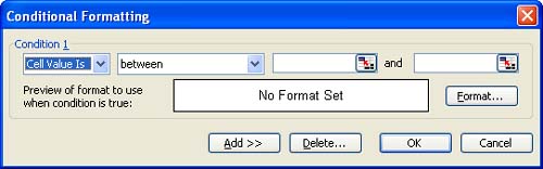
Another useful formatting feature that Excel provides is conditional formatting. Conditional formatting allows you to specify that certain results in the worksheet be formatted so that they stand out from the other entries in the worksheet. For example, if you wanted to track all the monthly sales figures that are below a certain amount, you can use conditional formatting to format them in red. Conditional formatting formats only cells that meet a certain condition.

To apply conditional formatting, follow these steps:

1. Select the cells to which you want to apply the conditional formatting.

2. Select the Format menu and select Conditional Formatting . The Conditional Formatting dialog box appears, as shown in Figure 10.4.

   Figure 10.4. Apply formats conditionally to highlight certain values.

   

3. Be sure that Cell Value Is is selected in the Condition 1 drop-down box on the left of the dialog box.

4. In the next drop-down box to the right, you select the condition. The default is Between. Other conditions include Equal To, Greater Than, Less Than, and other possibilities. Use the drop-down box to select the appropriate condition.

5. After selecting the condition, you must specify a cell or cells in the worksheet that Excel can use as a reference for the conditional formatting. For example, if you select Less Than as the condition, you must specify a cell in the worksheet that contains a value that can be used for comparison with the cells that you are applying the conditional formatting to. Click the Shrink button on the Conditional Formatting dialog box. You are returned to the worksheet. Select the reference cell for the condition.

6. Click the Expand button on the Conditional Formatting dialog box to expand the dialog box.

7. Now you can set the formatting that will be applied to cells that meet your condition. Click the Format button in the Conditional Formatting dialog box and select the formatting options for your condition in the Format Cells dialog box. Then click OK . Figure 10.5 shows a conditional format that applies bold and italic to values that are greater than the value contained in cell F8.

   Figure 10.5. Set the various options for your conditional formatting.

   

8. After setting the conditions to be met for conditional formatting (you can click Add to set more than one condition), click OK .

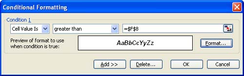
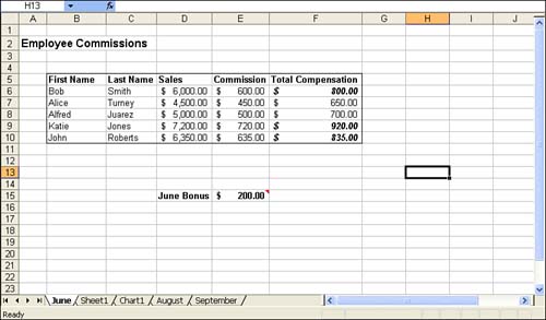
You are returned to the worksheet. Cells that meet the condition you set up for conditional formatting will be formatted with the options you specified. Figure 10.6 shows cells that the settings used in Figure 10.5 conditionally formatted.

Figure 10.6. Conditional formatting formats only the cells that meet your conditions.

Conditional Formatting Applied to Formulas You can also set up conditional formatting to highlight cells that contain a particular formula or function. Select Formula Is for Condition 1 in the Conditional Formatting dialog box and then type the formula or function in the box to the right.