Section 8.1. How Sound is Encoded
8.1. How Sound is EncodedThere are two parts to understanding how sound is encoded and manipulated.
8.1.1. The Physics of SoundPhysically, sounds are waves of air pressure. When something makes a sound, it makes ripples in the air just like stones or raindrops dropped into a pond cause ripples in the surface of the water (Figure 8.1). Each drop causes a wave of pressure to pass over the surface of the water, which causes visible rises in the water, and less visible but just as large depressions in the water. The rises are increases in pressure and the lows are decreases in pressure. Some of the ripples we see are actually ones that arise from combinations of ripplessome waves are the sums and interactions from other waves. Figure 8.1. Raindrops causing ripples in the surface of the water, just as sound causes ripples in the air.
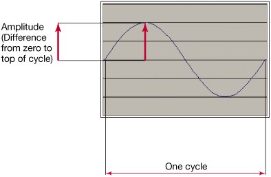
We call these increases in air pressure compressions and decreases in air pressure rarefactions. It's these compressions and rarefactions that lead to our hearing. The shape of the waves, their frequency, and their amplitude all impact how we perceive sound. The simplest sound in the world is a sine wave (Figure 8.2). In a sine wave, the compressions and rarefactions arrive with equal size and regularity. In a sine wave, one compression plus one rarefaction is called a cycle. The distance from the zero point to the greatest pressure (or least pressure) is called the amplitude. Figure 8.2. One cycle of the simplest sound, a sine wave.
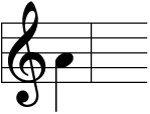
Formally, amplitude is measured in Newtons per meter-squared (N/m2). That's a rather hard unit to understand in terms of perception, but you can get a sense of the amazing range of human hearing from this unit. The smallest sound that humans typically hear is 0.0002N/m2, and the point at which we sense the vibrations in our entire body is 200N/m2! In general, amplitude is the most important factor in our perception of volume: If the amplitude rises, we typically perceive the sound as being louder. Other factors like air pressure factor into our perception of increased volume, too. Ever notice how sounds sound different on very humid days as compared with very dry days? When we perceive an increase in volume, we say that we're perceiving an increase in the intensity of sound. Intensity is measured in watts per meter-squared (W/m2). (Yes, those are watts just like the ones you're referring to when you get a 60-watt light bulbit's a measure of power.) The intensity is proportional to the square of the amplitude. For example, if the amplitude doubles, intensity quadruples. Human perception of sound is not a direct mapping from the physical reality. The study of the human perception of sound is called psychoacoustics. One of the odd facts about psychoacoustics is that most of our perception of sound is logarithmically related to the actual phenomena. Intensity is an example of this. A change in intensity from 0.1 W/m2 to 0.01 W/m2 sounds the same to us (as in the same amount of volume change) as a change in intensity of 0.001 W/m2 to 0.0001 W/m2. We measure the change in intensity in decibels (dB). That's probably the unit that you most often associate with volume. A decibel is a logarithmic measure, so it matches the way we perceive volume. It's always a ratio, a comparison of two values. 10 * log10(I1/I2) is the change in intensity in decibels between I1 and I2. If two amplitudes are measured under the same conditions, we can express the same definition as amplitudes: 20 * log10(A1/A2). If A2 = 2 * A1 (i.e., the amplitude doubles), the difference is roughly 6 dB. When decibel is used as an absolute measurement, it's in reference to the threshold of audibility at sound pressure level (SPL): 0 dB SPL. Normal speech has an intensity of about 60 dB SPL. Shouted speech is about 80 dB SPL. How often a cycle occurs is called the frequency. If a cycle is short, then there can be lots of them per second. If a cycle is long, then there are fewer of them. As the frequency increases we perceive that the pitch increases. We measure frequency in cycles per second (cps) or Hertz (Hz). All sounds are periodic: there is always some pattern of rarefaction and compression that leads to cycles. In a sine wave, the notion of a cycle is easy. In natural waves, it's not so clear where a pattern repeats. Even in the ripples in a pond, the waves aren't as regular as you might think. The time between peaks in waves isn't always the same: it varies. This means that a cycle may involve several peaks-and-valleys until it repeats. Humans hear between 2 Hz and 20,000 Hz (or 20 kilohertz, abbreviated 20 kHz). Again, as with amplitudes, that's an enormous range! To give you a sense of where music fits into that spectrum, the note A above middle C is 440 Hz in traditional, equal temperament tuning (Figure 8.3). Figure 8.3. The note A above middle C is 440 Hz.
Like intensity, our perception of pitch is almost exactly proportional to the log of the frequency. We really don't perceive absolute differences in pitch, but the ratio of the frequencies. If you heard a 100 Hz sound followed by a 200 Hz sound, you'd perceive the same pitch change (or pitch interval) as a shift from 1,000 Hz to 2,000 Hz. Obviously, a difference of 100 Hz is a lot smaller than a change of 1,000 Hz, but we perceive it to be the same. In standard tuning, the ratio in frequency between the same notes in adjacent octaves is 2:1. Frequency doubles each octave. We told you earlier that A above middle C is 440 Hz. You know then that the next A up the scale is 880 Hz. How we think about music is dependent upon our cultural standards, but there are some universals. Among these universals are the use of pitch intervals (e.g., the ratio between notes C and D remains the same in every octave), the relationship between octaves remains constant, and the existence of four to seven main pitches (not considering sharps and flats here) in an octave. What makes the experience of one sound different from another? Why is it that a flute playing a note sounds so different than a trumpet or a clarinet playing the same note? We still don't understand everything about psychoacoustics and what physical properties influence our perception of sound, but here are some of the factors that lead us to perceiving different sounds (especially musical instruments) as distinct.
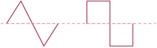
Figure 8.4. Some synthesizers using triangular (or sawtooth) or square waves.
8.1.2. Exploring SoundsOn your CD, you will find the MediaTools application with documentation for how to get it started. The MediaTools application contains tools for sound, graphics, and video. Using the sound tools, you can actually observe sounds as they're coming into your computer's microphone to get a sense of what louder and softer sounds look like, and what higher and lower pitched sounds look like. The basic sound editor looks like Figure 8.5. You can record sounds, open WAV files on your disk, and view the sounds in a variety of ways. (You will need a microphone on your computer to record sounds!) Figure 8.5. Sound editor main tool.
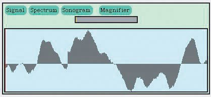
To view sounds, click the RECORD VIEWER button, then the RECORD button. (Hit the STOP button to stop recording.) There are three kinds of views that you can make of the sound. The first is the signal view (Figure 8.6). In the signal view, you're looking at the sound raweach increase in air pressure results in a rise in the graph, and each decrease in sound pressure results in a drop in the graph. Note how rapidly the wave changes! Try making some softer and louder sounds so that you can see how the look of the representation changes. You can always get back to the signal view from another view by clicking the SIGNAL button. Figure 8.6. Viewing the sound signal as it comes in. |


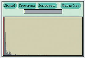
|

8.1.3. Encoding Sounds
You just read about how sounds work physically and how we perceive them. To manipulate these sounds on a computer and to play them back on a computer, we have to digitize them. To digitize sound means to take this flow of waves and turn it into numbers. We want to be able to capture a sound, perhaps manipulate it, and then play it back (through the computer's speakers) and hear what we capturedas exactly as possible.
The first part of the process of digitizing a sound is handled by the computer's hardwarethe physical machinery of the computer. If a computer has a microphone and the appropriate sound equipment (like a SoundBlaster sound card on Windows computers), then it's possible, at any moment, to measure the amount of air pressure against that microphone as a single number. Positive numbers correspond to rises in pressure, and negative numbers correspond to rarefactions. We call this an analog-to-digital conversion (ADC)we've moved from an analog signal (a continuously changing sound wave) to a digital value. This means that we can get an instantaneous measure of the sound pressure, but it's only one step along the way. Sound is a continuous changing pressure wave. How do we store that in our computer?
By the way, playback systems on computers work essentially the same in reverse. The sound hardware does a digital-to-analog conversion (DAC), and the analog signal is then sent to the speakers. The DAC process also requires numbers representing pressure.
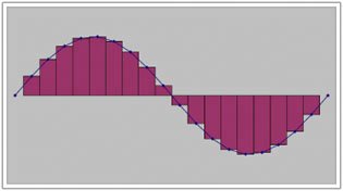
If you've had some calculus, you've got some idea of how we might do that. You know that we can get close to measuring the area under a curve with more and more rectangles whose height matches the curve (Figure 8.10). With that idea, it's pretty clear that if we capture enough of those microphone pressure readings, we capture the wave. We call each of those pressure readings a samplewe are literally "sampling" the sound at that moment. But how many samples do we need? In integral calculus, you compute the area under the curve by (conceptually) having an infinite number of rectangles. While computer memories are growing larger and larger all the time, we still can't capture an infinite number of samples per sound.
Figure 8.10. Area under a curve estimated with rectangles. (This item is displayed on page 260 in the print version)
Mathematicians and physicists wondered about these kinds of questions long before there were computers, and the answer to how many samples we need was actually computed long ago. The answer depends on the highest frequency you want to capture. Let's say that you don't care about any sounds higher than 8,000 Hz. The Nyquist theorem says that we would need to capture 16,000 samples per second to completely capture and define a wave whose frequency is less than 8,000 cycles per second.
|
This isn't just a theoretical result. The Nyquist theorem influences applications in our daily life. It turns out that human voices don't typically get over 4,000 Hz. That's why our telephone system is designed around capturing 8,000 samples per second. That's why playing music through the telephone doesn't really work very well. The limits of (most) human hearing is around 22,000 Hz. If we were to capture 44,000 samples per second, we would be able to capture any sound that we could actually hear. CD's are created by capturing sound at 44,100 samples per secondjust a little bit more than 44 kHz for technical reasons and for a fudge factor.
We call the rate at which samples are collected the sampling rate. Most sounds that we hear in daily life are well within the range of the limits of our hearing. You can capture and manipulate sounds in this class at a sampling rate of 22 kHz (22,000 samples per second), and it will sound quite reasonable. If you use a too low sampling rate to capture a high-pitched sound, you'll still hear something when you play the sound back, but the pitch will sound strange.
Typically, each of these samples are encoded in two bytes (16 bits). Though there are larger sample sizes, 16 bits works perfectly well for most applications. CD-quality sound uses 16 bit samples.
In 16 bits, the numbers that can be encoded range from -32,768 to 32,767. These aren't magic numbersthey make perfect sense when you understand the encoding. These numbers are encoded in 16 bits using a technique called two's complement notation, but we can understand it without knowing the details of that technique. We've got 16 bits to represent positive and negative numbers. Let's set aside one of those bits (remember, it's just 0 or 1) to represent whether we're talking about a positive (0) or negative (1) number. We call that the sign bit. That leaves 15 bits to represent the actual value. How many different patterns of 15 bits are there? We could start counting:
000000000000000 000000000000001 000000000000010 000000000000011 ... 111111111111110 111111111111111
That looks forbidding. Let's see if we can figure out a pattern. If we've got two bits, there are four patterns: 00, 01, 10, 11. If we've got three bits, there are eight patterns: 000, 001, 010, 011, 100, 101, 110, 111. It turns out that 22 is four, and 23 is eight. Play with four bits. How many patterns are there? 24 = 16. It turns out that we can state this as a general principle.
|
215 = 32,768. Why is there one more value in the negative range than the positive? Zero is neither negative nor positive, but if we want to represent it as bits, we need to define some pattern as zero. We use one of the positive range values (where the sign bit is zero) to represent zero, so that takes up one of the 32,768 patterns.
The sample size is a limitation on the amplitude of the sound that can be captured. If you have a sound that generates a pressure greater than 32,767 (or a rarefaction greater than 32,768), you'll only capture up to the limits of the 16 bits. If you were to look at the wave in the signal view, it would look like somebody took some scissors and clipped off the peaks of the waves. We call that effect clipping for that very reason. If you play (or generate) a sound that's clipped, it sounds badit sounds like your speakers are breaking.
There are other ways of digitizing sound, but this is by far the most common. The technical term for this way of encoding sound is pulse coded modulation (PCM). You may encounter that term if you read further in audio or play with audio software.
What this means is that a sound in a computer is a long list of numbers, each of which is a sample in time. There is an ordering in these samples: If you played the samples out of order, you wouldn't get the same sound at all. The most efficient way to store an ordered list of data items on a computer is with an array. An array is literally a sequence of bytes right next to one another in memory. We call each value in an array an element. We introduced arrays in Section 4.1.
We can easily store the samples that make up a sound in an array. Think of each two bytes as storing a single sample. The array will be largefor CD-quality sounds, there will be 44,100 elements for every second of recording. A minute long recording will result in an array with 26,460,000 elements.
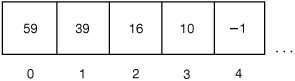
Each array element has a number associated with it, called its index. The index numbers start at 0 and increase sequentially. The first one is 0, the second one is 1, and so on. It may sound strange to say the index for the first array element is 0, but this is basically a measure of the distance from the first element in the array. Since the distance from the first element to itself is 0, the index is 0. You can think about an array as a long line of boxes, each one holding a value and each box having an index number on it (Figure 8.11).
Figure 8.11. A depiction of the first five elements in a real sound array.
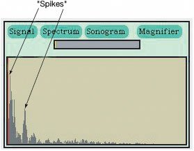
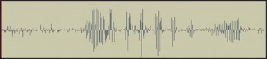
Using the MediaTools, you can graph a sound file (Figure 8.12) and get a sense of where the sound is quiet (small amplitudes), and loud (large amplitudes). This is actually important if you want to manipulate the sound. For example, the gaps between recorded words tend to be quietat least quieter than the words themselves. You can pick out where words end by looking for these gaps, as in Figure 8.12.
Figure 8.12. A sound recording graphed in the MediaTools.
You will soon read about how to read a file containing a recording of a sound into a sound object, view the samples in that sound, and change the values of the sound array elements. By changing the values in the array, you change the sound. Manipulating a sound is simply a matter of manipulating elements in an array.
EAN: N/A
Pages: 191