In this chapter, we will discuss database tables. We will look at the various types of tables and see when you might want to use each type; when one type of table is more appropriate than another. We will be concentrating on the physical storage characteristics of the tables; how the data is organized and stored.
Once upon a time, there was only one type of table really; a 'normal' table. It was managed in the same way a 'heap' is managed (the definition of which is below). Over time, Oracle added more sophisticated types of tables. There are clustered tables (two types of those), index organized tables, nested tables, temporary tables, and object tables in addition to the heap organized table. Each type of table has different characteristics that make it suitable for use in different application areas.
Types of Tables
We will define each type of table before getting into the details. There are seven major types of tables in Oracle 8i. They are:
Heap Organized Tables - This is a 'normal', standard database table. Data is managed in a heap-like fashion. As data is added, the first free space found in the segment that can fit the data will be used. As data is removed from the table, it allows space to become available for reuse by subsequent INSERTs and UPDATEs. This is the origin of the name heap as it refers to tables like this. A heap is a bunch of space and it is used in a somewhat random fashion.
Index Organized Tables - Here, a table is stored in an index structure. This imposes physical order on the rows themselves. Whereas in a heap, the data is stuffed wherever it might fit, in an index organized table the data is stored in sorted order, according to the primary key.
Clustered Tables - Two things are achieved with these. First, many tables may be stored physically joined together. Normally, one would expect data from only one table to be found on a database block. With clustered tables, data from many tables may be stored together on the same block. Secondly, all data that contains the same cluster key value will be physically stored together. The data is 'clustered' around the cluster key value. A cluster key is built using a B*Tree index.
Hash Clustered Tables - Similar to the clustered table above, but instead of using a B*Tree index to locate the data by cluster key, the hash cluster hashes the key to the cluster, to arrive at the database block the data should be on. In a hash cluster the data is the index (metaphorically speaking). This would be appropriate for data that is read frequently via an equality comparison on the key.
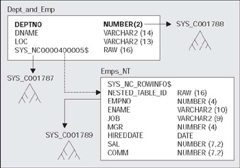
Nested Tables - These are part of the Object Relational extensions to Oracle. They are simply system generated and maintained child tables in a parent/child relationship. They work much in the same way as EMP and DEPT in the SCOTT schema. EMP is considered to be a child of the DEPT table, since the EMP table has a foreign key, DEPTNO, that points to DEPT. The main difference is that they are not 'standalone' tables like EMP.
Temporary Tables - These tables store scratch data for the life of a transaction or the life of a session. These tables allocate temporary extents as needed from the users temporary tablespace. Each session will only see the extents it allocates and never sees any of the data created in any other session.
Object Tables - These are tables that are created based on an object type. They are have special attributes not associated with non-object tables, such as a system generated REF (object identifier) for each row. Object tables are really special cases of heap, index organized, and temporary tables, and may include nested tables as part of their structure as well.
In general, there are a couple of facts about tables, regardless of their type. Some of these are:
A table can have up to 1,000 columns, although I would recommend against a design that does, unless there was some pressing need. Tables are most efficient with far fewer than 1,000 columns.
A table can have a virtually unlimited number of rows. Although you will hit other limits that prevent this from happening. For example, a tablespace can have at most 1,022 files typically. Say you have 32 GB files, that is to say 32,704 GB per tablespace. This would be 2,143,289,344 blocks, each of which are 16 KB in size. You might be able to fit 160 rows of between 80 to 100 bytes per block. This would give you 342,926,295,040 rows. If we partition the table though, we can easily multiply this by ten times or more. There are limits, but you'll hit other practical limitations before even coming close to these figures.
A table can have as many indexes as there are permutations of columns, taken 32 at a time (and permutations of functions on those columns), although once again practical restrictions will limit the actual number of indexes you will create and maintain.
There is no limit to the number of tables you may have. Yet again, practical limits will keep this number within reasonable bounds. You will not have millions of tables (impracticable to create and manage), but thousands of tables, yes.
We will start with a look at some of the parameters and terminology relevant to tables and define them. After that we'll jump into a discussion of the basic 'heap organized' table and then move onto the other types.
Terminology
In this section, we will cover the various storage parameters and terminology associated with tables. Not all parameters are used for every table type. For example, the PCTUSED parameter is not meaningful in the context of an index organized table. We will mention in the discussion of each table type below which parameters are relevant. The goal is to introduce the terms and define them. As appropriate, more information on using specific parameters will be covered in subsequent sections.
High Water Mark
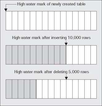
This is a term used with objects stored in the database. If you envision a table for example as a 'flat' structure, as a series of blocks laid one after the other in a line from left to right, the highwatermark would be the right most block that ever contained data. For example:
This shows that the high water mark starts at the first block of a newly created table. As data is placed into the table over time and more blocks get used, the high water mark rises. If we delete some (or even all) of the rows in the table, we might have many blocks that no longer contain data, but they are still under the high water mark and will remain under the high water mark until the object is rebuilt or truncated.
The high water mark is relevant since Oracle will scan all blocks under the high water mark, even when they contain no data, during a full scan. This will impact the performance of a full scan - especially if most of the blocks under the high water mark are empty. To see this, just create a table with 1,000,000 rows (or create any table with a large number of rows). Do a SELECTCOUNT(*) from this table. Now, DELETE every row in it and you will find that the SELECTCOUNT(*) takes just as long to count zero rows as it did to count 1,000,000. This is because Oracle is busy reading all of the blocks below the high water mark to see if they contain data. You should compare this to what happens if you used TRUNCATE on the table instead of deleting each individual row. TRUNCATE will reset the high water mark of a table back to 'zero'. If you plan on deleting every row in a table, TRUNCATE would be the method of my choice for this reason.
FREELISTS
The FREELIST is where Oracle keeps tracks of blocks under the high water mark for objects that have free space on them. Each object will have at least one FREELIST associated with it and as blocks are used, they will be placed on or taken off of the FREELIST as needed. It is important to note that only blocks under the high water mark of an object will be found on the FREELIST. The blocks that remain above the high water mark, will be used only when the FREELISTs are empty, at which point Oracle advances the high water mark and adds these blocks to the FREELIST. In this fashion, Oracle postpones increasing the high water mark for an object until it has to.
An object may have more than one FREELIST. If you anticipate heavy INSERT or UPDATE activity on an object by many concurrent users, configuring more then one FREELIST can make a major positive impact on performance (at the cost of possible additional storage). As we will see later, having sufficient FREELISTs for your needs is crucial.
Freelists can be a huge positive performance influence (or inhibitor) in an environment with many concurrent inserts and updates. An extremely simple test can show the benefits of setting this correctly. Take the simplest table in the world:
tkyte@TKYTE816> create table t ( x int );
and using two sessions, start inserting into it like wild. If you measure the system-wide wait events for block related waits before and after, you will find huge waits, especially on data blocks (trying to insert data). This is frequently caused by insufficient FREELISTs on tables (and on indexes but we'll cover that again in Chapter 7, Indexes). For example, I set up a temporary table:
tkyte@TKYTE816> create global temporary table waitstat_before 2 on commit preserve rows 3 as 4 select * from v$waitstat 5 where 1=0 6 /Table created.
to hold the before picture of waits on blocks. Then, in two sessions, I simultaneously ran:
tkyte@TKYTE816> truncate table waitstat_before;Table truncated.tkyte@TKYTE816> insert into waitstat_before 2 select * from v$waitstat 3 /14 rows created.tkyte@TKYTE816> begin 2 for i in 1 .. 100000 3 loop 4 insert into t values ( i ); 5 commit; 6 end loop; 7 end; 8/PL/SQL procedure successfully completed.
Now, this is a very simple block of code, and we are the only users in the database here. We should get as good performance as you can get. I've plenty of buffer cache configured, my redo logs are sized appropriately, indexes won't be slowing things down; this should run fast. What I discover afterwards however, is that:
tkyte@TKYTE816> select a.class, b.count-a.count count, b.time-a.time time 2 from waitstat_before a, v$waitstat b 3 where a.class = b.class 4 /CLASS COUNT TIME------------------ ---------- ----------bitmap block 0 0bitmap index block 0 0data block 4226 3239extent map 0 0free list 0 0save undo block 0 0save undo header 0 0segment header 2 0sort block 0 0system undo block 0 0system undo header 0 0undo block 0 0undo header 649 36unused 0 0
I waited over 32 seconds during these concurrent runs. This is entirely due to not having enough FREELISTs configured on my tables for the type of concurrent activity I am expecting to do. I can remove all of that wait time easily, just by creating the table with multiple FREELISTs:
tkyte@TKYTE816> create table t ( x int ) storage ( FREELISTS 2 );Table created.
or by altering the object:
tkyte@TKYTE816> alter table t storage ( FREELISTS 2 );Table altered.
You will find that both wait events above go to zero; it is that easy. What you want to do for a table is try to determine the maximum number of concurrent (truly concurrent) inserts or updates that will require more space. What I mean by truly concurrent, is how often do you expect two people at exactly the same instant, to request a free block for that table. This is not a measure of overlapping transactions, it is a measure of sessions doing an insert at the same time, regardless of transaction boundaries. You want to have about as many FREELISTs as concurrent inserts into the table to increase concurrency.
You should just set FREELISTs really high and then not worry about it, right? Wrong - of course, that would be too easy. Each process will use a single FREELIST. It will not go from FREELIST to FREELIST to find space. What this means is that if you have ten FREELISTs on a table and the one your process is using exhausts the free buffers on its list, it will not go to another list for space. It will cause the table to advance the high water mark, or if the tables high water cannot be advanced (all space is used), to extend, to get another extent. It will then continue to use the space on its FREELIST only (which is empty now). There is a tradeoff to be made with multiple FREELISTs. On one hand, multiple FREELISTs is a huge performance booster. On the other hand, it will probably cause the table to use more disk space then absolutely necessary. You will have to decide which is less bothersome in your environment.
Do not underestimate the usefulness of this parameter, especially since we can alter it up and down at will with Oracle 8.1.6 and up. What you might do is alter it to a large number to perform some load of data in parallel with the conventional path mode of SQLLDR. You will achieve a high degree of concurrency for the load with minimum waits. After the load, you can alter the FREELISTs back down to some, more day-to-day, reasonable number, the blocks on the many existing FREELISTs will be merged into the one master FREELIST when you alter the space down.
PCTFREE and PCTUSED
These two settings control when blocks will be put on and taken off the FREELISTs. When used with a table (but not an Index Organized Table as we'll see), PCTFREE tells Oracle how much space should be reserved on a block for future updates. By default, this is 10 percent. What this means is that if we use an 8 KB block size, as soon as the addition of a new row onto a block would cause the free space on the block to drop below about 800 bytes, Oracle will use a new block instead of the existing block. This 10 percent of the data space on the block is set aside for updates to the rows on that block. If we were to update them - the block would still be able to hold the updated row.
Now, whereas PCTFREE tells Oracle when to take a block off the FREELIST making it no longer a candidate for insertion, PCTUSED tells Oracle when to put a block on the FREELIST again. If the PCTUSED is set to 40 percent (the default), and the block hit the PCTFREE level (it is not on the FREELIST currently), then 61 percent of the block must be free space before Oracle will put the block back on the FREELIST. If we are using the default values for PCTFREE (10) and PCTUSED (40) then a block will remain on the FREELIST until it is 90 percent full (10 percent free space). Once it hits 90 percent, it will be taken off of the FREELIST and remain off the FREELIST, until the free space on the block exceeds 60 percent of the block.
Pctfree and PCTUSED are implemented differently for different table types as will be noted below when we discuss each type. Some table types employ both, others only use PCTFREE and even then only when the object is created.
There are three settings for PCTFREE, too high, too low, and just about right. If you set PCTFREE for blocks too high, you will waste space. If you set PCTFREE to 50 percent and you never update the data, you have just wasted 50 percent of every block. On another table however, 50 percent may be very reasonable. If the rows start out small and tend to double in size, a large setting for PCTFREE will avoid row migration.
Row Migration
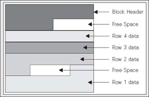
So, that poses the question; what exactly is row migration? Row migration is when a row is forced to leave the block it was created on, because it grew too large to fit on that block with the rest of the rows. I'll illustrate a row migration below. We start with a block that looks like this:
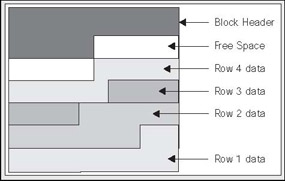
Approximately one seventh of the block is free space. However, we would like to more than double the amount of space used by row 4 via an UPDATE (it currently consumes a seventh of the block). In this case, even if Oracle coalesced the space on the block like this:
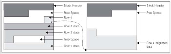
there is still insufficient room to grow row 4 by more than two times its current size, because the size of the free space is less than the size of row 4. If the row could have fitted in the coalesced space, then this would have happened. This time however, Oracle will not perform this coalescing and the block will remain as it is. Since row 4 would have to span more than one block if it stayed on this block, Oracle will move, or migrate, the row. However, it cannot just move it; it must leave behind a 'forwarding address'. There may be indexes that physically point to this address for row 4. A simple update will not modify the indexes as well (note that there is a special case with partitioned tables that a row ID, the address of a row, will change. We will look at this case in the Chapter 14 on Partitioning,). Therefore, when Oracle migrates the row, it will leave behind a pointer to where the row really is. After the update, the blocks might look like the following:
So, this is what a migrated row is; it is a row that had to move from the block it was inserted into, onto some other block. Why is this an issue? Your application will never know, the SQL you use is no different. It only matters for performance reasons. If we go to read this row via an index, the index will point to the original block. That block will point to the new block. Instead of doing the two or so I/Os to read the index plus one I/O to read the table, we'll need to do yet one more I/O to get to the actual row data. In isolation, this is no 'big deal'; you won't even notice this. However, when you have a sizable percentage of your rows in this state with lots of users you will begin to notice this side effect. Access to this data will start to slow down (additional I/Os add to the access time), your buffer cache efficiency goes down (you need to buffer twice the amount of blocks you would if they were not migrated), and your table grows in size and complexity. It is for these reasons that you do not want migrated rows. It is interesting to note what Oracle will do if the row that was migrated from the block on the left to the block on the right, in the diagram above, was to have to migrate again at some future point in time. This would be due to other rows being added to the block it was migrated to and then updating this row to make it even larger. Oracle will actually migrate the row back to the original block and if there is sufficient space leave it there (the row might become 'un-migrated'). If there isn't sufficient space, Oracle will migrate the row to another block all together and change the forwarding address on the original block. As such, row migrations will always involve one level of indirection. So, now we are back to PCTFREE and what it is used for; it is the setting that will help you to minimize row chaining when set properly.
Setting PCTFREE and PCTUSED values
Setting PCTFREE and PCTUSED is an important, and a greatly overlooked, topic, I would like to show you how you can measure the behavior of your objects, to see how space is being used. I will use a stored procedure that will show the effects of inserts on a table with various PCTFREE/PCTUSED settings followed by a series of updates to the same data. This will illustrate how these settings can affect the number of blocks available on the FREELIST (which ultimately will affect how space is used, how many rows are migrated and so on). These scripts are illustrative; they don't tell you what to set the values to, they can be used by you to figure out how Oracle is treating your blocks given various types of updates. They are templates that you will have to modify in order to effectively use them.
I started by creating a test table:
tkyte@TKYTE816> create table t ( x int, y char(1000) default 'x' );Table created.
It is a very simple table but for illustrative purposes will serve nicely. By using the CHAR type, I've ensured every row with a non-null value for Y will be 1,000 bytes long. I should be able to 'guess' how things will work given a specific block size. Now for the routine to measure FREELIST and block usage:
tkyte@TKYTE816> create or replace procedure measure_usage 2 as 3 l_free_blks number; 4 l_total_blocks number; 5 l_total_bytes number; 6 l_unused_blocks number; 7 l_unused_bytes number; 8 l_LastUsedExtFileId number; 9 l_LastUsedExtBlockId number; 10 l_LAST_USED_BLOCK number; 11 12 procedure get_data 13 is 14 begin 15 dbms_space.free_blocks 16 ( segment_owner => USER, 17 segment_name => 'T', 18 segment_type => 'TABLE', 19 FREELIST_group_id => 0, 20 free_blks => l_free_blks ); 21 22 dbms_space.unused_space 23 ( segment_owner => USER, 24 segment_name => 'T', 25 segment_type => 'TABLE', 26 total_blocks => l_total_blocks, 27 total_bytes => l_total_bytes, 28 unused_blocks => l_unused_blocks, 29 unused_bytes => l_unused_bytes, 30 LAST_USED_EXTENT_FILE_ID => l_LastUsedExtFileId, 31 LAST_USED_EXTENT_BLOCK_ID => l_LastUsedExtBlockId, 32 LAST_USED_BLOCK => l_last_used_block ) ; 33 34 35 dbms_output.put_line( L_free_blks || ' on FREELIST, ' || 36 to_number(l_total_blocks-l_unused_blocks-1 ) || 37 ' used by table' ); 38 end; 39 begin 40 for i in 0 .. 10 41 loop 42 dbms_output.put( 'insert ' || to_char(i,'00') || ' ' ); 43 get_data; 44 insert into t (x) values ( i ); 45 commit ; 46 end loop; 47 48 49 for i in 0 .. 10 50 loop 51 dbms_output.put( 'update ' || to_char(i,'00') || ' ' ); 52 get_data; 53 update t set y = null where x = i; 54 commit; 55 end loop; 56 end; 57 /Procedure created.
Here we use two routines in the DBMS_SPACE package that tell us how many blocks are on a segment's FREELIST, how many blocks are allocated to the table, unused blocks and so on. We can use this information to tell ourselves how many of the blocks that have been used by the table (below the high water mark of the table) are on the FREELIST. I then insert 10 rows into the table with a non-Null Y. Then I come back and update Y to Null row by row. Given that I have an 8 KB block size, with a default PCTFREE of 10 and a default PCTUSED of 40, I would expect that seven rows should fit nicely on the block (the calculation below is done without considering the block/row overhead):
(2+1)bytes for X + (1000+2)bytes for Y = 10051005 bytes/row * 7 rows = 70358192 - 7035 bytes (blocksize) = 1157 bytes1157 bytes are leftover, insufficient for another row plus 800+ bytes (10% of theblock)
Now, since 10 percent of the 8 KB block is about 800 + bytes, we know we cannot fit another row onto that block. If we wanted to, we could calculate the block header exactly, here we will just guess that it is less then 350 + bytes (1157 - 800 = 357). That gives us room for seven rows per block.
Next estimate how many updates it will take to put a block back on the FREELIST. Here, we know the block must be less than 40 percent used - that is only a maximum of 3,275 bytes can be in use to get back onto the free list. We would expect then that if each UPDATE gives back 1,000 bytes, it would take about four UPDATEs to put a block back on the FREELIST. Well, lets see how well I did:
tkyte@TKYTE816> exec measure_usage;insert 00 0 on FREELIST, 0 used by tableinsert 01 1 on FREELIST, 1 used by tableinsert 02 1 on FREELIST, 1 used by tableinsert 03 1 on FREELIST, 1 used by tableinsert 04 1 on FREELIST, 1 used by tableinsert 05 1 on FREELIST, 1 used by tableinsert 06 1 on FREELIST, 1 used by tableinsert 07 1 on FREELIST, 1 used by table -- between the 7th and 8th rowsinsert 08 1 on FREELIST, 2 used by table we added another block 'in use'insert 09 1 on FREELIST, 2 used by tableinsert 10 1 on FREELIST, 2 used by tableupdate 00 1 on FREELIST, 2 used by tableupdate 01 1 on FREELIST, 2 used by tableupdate 02 1 on FREELIST, 2 used by tableupdate 03 1 on FREELIST, 2 used by tableupdate 04 2 on FREELIST, 2 used by table -- the 4th update put anotherupdate 05 2 on FREELIST, 2 used by table block back on the free listupdate 06 2 on FREELIST, 2 used by tableupdate 07 2 on FREELIST, 2 used by tableupdate 08 2 on FREELIST, 2 used by tableupdate 09 2 on FREELIST, 2 used by tableupdate 10 2 on FREELIST, 2 used by tablePL/SQL procedure successfully completed.
Sure enough, after seven INSERTs, another block is added to the table. Likewise, after four UPDATEs, the blocks on the FREELIST increase from 1 to 2 (both blocks are back on the FREELIST, available for INSERTs). If we drop and recreate the table T with different settings and then measure it again, we get the following:
tkyte@TKYTE816> create table t ( x int, y char(1000) default 'x' ) pctfree 10 2 pctused 80;Table created.tkyte@TKYTE816> exec measure_usage;insert 00 0 on FREELIST, 0 used by tableinsert 01 1 on FREELIST, 1 used by tableinsert 02 1 on FREELIST, 1 used by tableinsert 03 1 on FREELIST, 1 used by tableinsert 04 1 on FREELIST, 1 used by tableinsert 05 1 on FREELIST, 1 used by tableinsert 06 1 on FREELIST, 1 used by tableinsert 07 1 on FREELIST, 1 used by tableinsert 08 1 on FREELIST, 2 used by tableinsert 09 1 on FREELIST, 2 used by tableinsert 10 1 on FREELIST, 2 used by tableupdate 00 1 on FREELIST, 2 used by tableupdate 01 2 on FREELIST, 2 used by table -- first update put a blockupdate 02 2 on FREELIST, 2 used by table back on the free list due to theupdate 03 2 on FREELIST, 2 used by table much higher pctusedupdate 04 2 on FREELIST, 2 used by tableupdate 05 2 on FREELIST, 2 used by tableupdate 06 2 on FREELIST, 2 used by tableupdate 07 2 on FREELIST, 2 used by tableupdate 08 2 on FREELIST, 2 used by tableupdate 09 2 on FREELIST, 2 used by tableupdate 10 2 on FREELIST, 2 used by tablePL/SQL procedure successfully completed.
We can see the effect of increasing PCTUSED here. The very first UPDATE had the effect of putting the block back on the FREELIST. That block can be used by another INSERT again that much faster.
Does that mean you should increase your PCTUSED? No, not necessarily. It depends on how your data behaves over time. If your application goes through cycles of:
Adding data (lots of INSERTs) followed by,
UPDATEs - Updating the data causing the rows to grow and shrink.
Go back to adding data.
I might never want a block to get put onto the FREELIST as a result of an update. Here we would want a very low PCTUSED, causing a block to go onto a FREELIST only after all of the row data has been deleted. Otherwise, some of the blocks that have rows that are temporarily 'shrunken' would get newly inserted rows if PCTUSED was set high. Then, when we go to update the old and new rows on these blocks; there won't be enough room for them to grow and they migrate.
In summary, PCTUSED and PCTFREE are crucial. On one hand you need to use them to avoid too many rows from migrating, on the other hand you use them to avoid wasting too much space. You need to look at your objects, describe how they will be used, and then you can come up with a logical plan for setting these values. Rules of thumb may very well fail us on these settings; they really need to be set based on how you use it. You might consider (and remember high and low are relative terms):
High PCTFREE, Low PCTUSED - For when you insert lots of data that will be updated and the updates will increase the size of the rows frequently. This reserves a lot of space on the block after inserts (high PCTFREE) and makes it so that the block must almost be empty before getting back onto the free list (low PCTUSED).
Low PCTFREE, High PCTUSED - If you tend to only ever INSERT or DELETE from the table or if you do UPDATE, the UPDATE tends to shrink the row in size.
INITIAL, NEXT, and PCTINCREASE
These are storage parameters that define the size of the INITIAL and subsequent extents allocated to a table and the percentage by which the NEXT extent should grow. For example, if you use an INITIAL extent of 1 MB, a NEXT extent of 2 MB, and a PCTINCREASE of 50 - your extents would be:
1 MB.
2 MB.
3 MB (150 percent of 2).
4.5 MB (150 percent of 3).
and so on. I consider these parameters to be obsolete. The database should be using locally managed tablespaces with uniform extent sizes exclusively. In this fashion the INITIAL extent is always equal to the NEXT extent size and there is no such thing as PCTINCREASE - a setting that only causes fragmentation in a tablespace.
In the event you are not using locally managed tablespaces, my recommendation is to always set INITIAL=NEXT and PCTINCREASE to ZERO. This mimics the allocations you would get in a locally managed tablespace. All objects in a tablespace should use the same extent allocation strategy to avoid fragmentation.
MINEXTENTS and MAXEXTENTS
These settings control the number of extents an object may allocate for itself. The setting for MINEXTENTS tells Oracle how many extents to allocate to the table initially. For example, in a locally managed tablespace with uniform extent sizes of 1 MB, a MINEXTENTS setting of 10 would cause the table to have 10 MB of storage allocated to it.
MAXEXTENTS is simply an upper bound on the possible number of extents this object may acquire. If you set MAXEXTENTS to 255 in that same tablespace, the largest the table would ever get to would be 255 MB in size. Of course, if there is not sufficient space in the tablespace to grow that large, the table will not be able to allocate these extents.
LOGGING and NOLOGGING
Normally objects are created in a LOGGING fashion, meaning all operations performed against them that can generate redo will generate it. NOLOGGING allows certain operations to be performed against that object without the generation of redo. NOLOGGING only affects only a few specific operations such as the initial creation of the object, or direct path loads using SQLLDR, or rebuilds (see the SQL Language Reference Manual for the database object you are working with to see which operations apply).
This option does not disable redo log generation for the object in general; only for very specific operations. For example, if I create a table as SELECTNOLOGGING and then, INSERTINTOTHAT_TABLEVALUES(1), the INSERT will be logged, but the table creation would not have been.
INITRANS and MAXTRANS
Each block in an object has a block header. Part of this block header is a transaction table, entries will be made in the transaction table to describe which transactions have what rows/elements on the block locked. The initial size of this transaction table is specified by the INITRANS setting for the object. For tables this defaults to 1 (indexes default to 2). This transaction table will grow dynamically as needed up to MAXTRANS entries in size (given sufficient free space on the block that is). Each allocated transaction entry consumes 23 bytes of storage in the block header.
Heap Organized Table
A heap organized table is probably used 99 percent (or more) of the time in applications, although that might change over time with the advent of index organized tables, now that index organized tables can themselves be indexed. A heap organized table is the type of table you get by default when you issue the CREATETABLE statement. If you want any other type of table structure, you would need to specify that in the CREATE statement itself.
A heap is a classic data structure studied in computer science. It is basically, a big area of space, disk, or memory (disk in the case of a database table, of course), which is managed in an apparently random fashion. Data will be placed where it fits best, not in any specific sort of order. Many people expect data to come back out of a table in the same order it was put into it, but with a heap, this is definitely not assured. In fact, rather the opposite is guaranteed; the rows will come out in a wholly unpredictable order. This is quite easy to demonstrate. I will set up a table, such that in my database I can fit one full row per block (I am using an 8 KB block size). You do not need to have the case where you only have one row per block I am just taking advantage of that to demonstrate a predictable sequence of events. The following behavior will be observed on tables of all sizes, in databases with any blocksize:
tkyte@TKYTE816> create table t 2 ( a int, 3 b varchar2(4000) default rpad('*',4000,'*'), 4 c varchar2(3000) default rpad('*',3000,'*') 5 ) 6 /Table created.tkyte@TKYTE816> insert into t (a) values ( 1);1 row created.tkyte@TKYTE816> insert into t (a) values ( 2);1 row created.tkyte@TKYTE816> insert into t (a) values ( 3);1 row created.tkyte@TKYTE816> delete from t where a = 2 ;1 row deleted.tkyte@TKYTE816> insert into t (a) values ( 4);1 row created.tkyte@TKYTE816> select a from t; A---------- 1 4 3
Adjust columns B and C to be appropriate for your block size if you would like to reproduce this. For example, if you have a 2 KB block size, you do not need column C, and column B should be a VARCHAR2(1500) with a default of 1500 asterisks. Since data is managed in a heap in a table like this, as space becomes available, it will be reused. A full scan of the table will retrieve the data as it hits it, never in the order of insertion. This is a key concept to understand about database tables; in general, they are inherently unordered collections of data. You should also note that we do not need to use a DELETE in order to observe the above - I could achieve the same results using onlyINSERTs. If I insert a small row, followed by a very large row that will not fit on the block with the small row, and then a small row again, I may very well observe that the rows come out by default in the order 'small row, small row, large row'. They will not be retrieved in the order of insertion. Oracle will place the data where it fits, not in any order by date or transaction.
If your query needs to retrieve data in order of insertion, we must add a column to that table that we can use to order the data when retrieving it. That column could be a number column for example that was maintained with an increasing sequence (using the Oracle SEQUENCE object). We could then approximate the insertion order using 'select by ordering' on this column. It will be an approximation because the row with sequence number 55 may very well have committed before the row with sequence 54, therefore it was officially 'first' in the database.
So, you should just think of a heap organized table as a big, unordered collection of rows. These rows will come out in a seemingly random order and depending on other options being used (parallel query, different optimizer modes and so on), may come out in a different order with the same query. Do not ever count on the order of rows from a query unless you have an ORDERBY statement on your query!
That aside, what is important to know about heap tables? Well, the CREATETABLE syntax spans almost 40 pages in the SQL reference manual provided by Oracle so there are lots of options that go along with them. There are so many options that getting a hold on all of them is pretty difficult. The 'wire diagrams' (or 'train track' diagrams) alone take eight pages to cover. One trick I use to see most of the options available to me in the create table statement for a given table, is to create the table as simply as possible, for example:
tkyte@TKYTE816> create table t 2 ( x int primary key , 3 y date, 4 z clob ) 5 /Table created.
Then using the standard export and import utilities (see Chapter 8 on Import and Export), we'll export the definition of it and have import show us the verbose syntax:
I'll now find that T.SQL contains my CREATE table statement in its most verbose form, I've formatted it a bit for easier reading but otherwise it is straight from the DMP file generated by export:
The nice thing about the above is that it shows many of the options for my CREATETABLE statement. I just have to pick data types and such; Oracle will produce the verbose version for me. I can now customize this verbose version, perhaps changing the ENABLESTORAGEINROW to DISABLESTORAGEINROW - this would disable the stored of the LOB data in the row with the structured data, causing it to be stored in another segment. I use this trick myself all of the time to save the couple minutes of confusion I would otherwise have if I tried to figure this all out from the huge wire diagrams. I can also use this to learn what options are available to me on the CREATETABLE statement under different circumstances.
This is how I figure out what is available to me as far as the syntax of the CREATETABLE goes - in fact I use this trick on many objects. I'll have a small testing schema, create 'bare bones' objects in that schema, export using OWNER=THAT_SCHEMA, and do the import. A review of the generated SQL file shows me what is available.
Now that we know how to see most of the options available to us on a given CREATETABLE statement, what are the important ones we need to be aware of for heap tables? In my opinion they are:
FREELISTS - every table manages the blocks it has allocated in the heap on a FREELIST. A table may have more then one FREELIST. If you anticipate heavy insertion into a table by many users, configuring more then one FREELIST can make a major positive impact on performance (at the cost of possible additional storage). Refer to the previous discussion and example above (in the section FREELISTS) for the sort of impact this setting can have on performance.
PCTFREE - a measure of how full a block can be made during the INSERT process. Once a block has less then the 'PCTFREE' space left on it, it will no longer be a candidate for insertion of new rows. This will be used to control row migrations caused by subsequent updates and needs to be set based on how you use the table.
PCTUSED - a measure of how empty a block must become, before it can be a candidate for insertion again. A block that has less then PCTUSED space used is a candidate for insertion of new rows. Again, like PCTFREE, you must consider how you will be using your table in order to set this appropriately.
INITRANS - the number of transaction slots initially allocated to a block. If set too low (defaults to 1) this can cause concurrency issues in a block that is accessed by many users. If a database block is nearly full and the transaction list cannot be dynamically expanded - sessions will queue up waiting for this block as each concurrent transaction needs a transaction slot. If you believe you will be having many concurrent updates to the same blocks, you should consider increasing this value
Note: LOB data that is stored out of line in the LOB segment does not make use of the PCTFREE/PCTUSED parameters set for the table. These LOB blocks are managed differently. They are always filled to capacity and returned to the FREELIST only when completely empty.
These are the parameters you want to pay particularly close attention to. I find that the rest of the storage parameters are simply not relevant any more. As I mentioned earlier in the chapter, we should use locally managed tablespaces, and these do not utilize the parameters PCTINCREASE, NEXT, and so on.
Index Organized Tables
Index organized tables (IOTs) are quite simply a table stored in an index structure. Whereas a table stored in a heap is randomly organized, data goes wherever there is available space, data in an IOT is stored and sorted by primary key. IOTs behave just like a 'regular' table does as far as your application is concerned; you use SQL to access it as normal. They are especially useful for information retrieval (IR), spatial, and OLAP applications.
What is the point of an IOT? One might ask the converse actually; what is the point of a heap-organized table? Since all tables in a relational database are supposed to have a primary key anyway, isn't a heap organized table just a waste of space? We have to make room for both the table and the index on the primary key of the table when using a heap organized table. With an IOT, the space overhead of the primary key index is removed, as the index is the data, the data is the index. Well, the fact is that an index is a complex data structure that requires a lot of work to manage and maintain. A heap on the other hand is trivial to manage by comparison. There are efficiencies in a heap-organized table over an IOT. That said, there are some definite advantages to IOTs over their counterpart the heap. For example, I remember once building an inverted list index on some textual data (this predated the introduction of interMedia and related technologies). I had a table full of documents. I would parse the documents and find words within the document. I had a table that then looked like this:
create table keywords( word varchar2(50), position int, doc_id int, primary key(word,position,doc_id));
Here I had a table that consisted solely of columns of the primary key. I had over 100 percent overhead; the size of my table and primary key index were comparable (actually the primary key index was larger since it physically stored the row ID of the row it pointed to whereas a row ID is not stored in the table - it is inferred). I only used this table with a WHERE clause on the WORD or WORD and POSITION columns. That is, I never used the table; I only used the index on the table. The table itself was no more then overhead. I wanted to find all documents containing a given word (or 'near' another word and so on). The table was useless, it just slowed down the application during maintenance of the KEYWORDS table and doubled the storage requirements. This is a perfect application for an IOT.
Another implementation that begs for an IOT is a code lookup table. Here you might have ZIP_CODE to STATE lookup for example. You can now do away with the table and just use the IOT itself. Anytime you have a table, which you access via its primary key frequently it is a candidate for an IOT.
Another implementation that makes good use of IOTs is when you want to build your own indexing structure. For example, you may want to provide a case insensitive search for your application. You could use function-based indexes (see Chapter 7 on Indexes for details on what this is). However, this feature is available with Enterprise and Personal Editions of Oracle only. Suppose you have the Standard Edition, one way to provide a case insensitive, keyword search would be to 'roll your own' function-based index. For example, suppose you wanted to provide a case-insensitive search on the ENAME column of the EMP table. One approach would be to create another column, ENAME_UPPER, in the EMP table and index that column. This shadow column would be maintained via a trigger. If you didn't like the idea of having the extra column in the table, you can just create your own function-based index, with the following:
tkyte@TKYTE816> create table emp as select * from scott.emp;Table created.tkyte@TKYTE816> create table upper_ename 2 ( x$ename, x$rid, 3 primary key (x$ename,x$rid) 4 ) 5 organization index 6 as 7 select upper(ename), rowid from emp 8 /Table created.tkyte@TKYTE816> create or replace trigger upper_ename 2 after insert or update or delete on emp 3 for each row 4 begin 5 if (updating and (:old.ename||'x' <> :new.ename||'x')) 6 then 7 delete from upper_ename 8 where x$ename = upper(:old.ename) 9 and x$rid = :old.rowid; 10 11 insert into upper_ename 12 (x$ename,x$rid) values 13 ( upper(:new.ename), :new.rowid ); 14 elsif (inserting) 15 then 16 insert into upper_ename 17 (x$ename,x$rid) values 18 ( upper(:new.ename), :new.rowid ); 19 elsif (deleting) 20 then 21 delete from upper_ename 22 where x$ename = upper(:old.ename) 23 and x$rid = :old.rowid; 24 end if; 25 end; 26 /Trigger created.tkyte@TKYTE816> update emp set ename = initcap(ename);14 rows updated.tkyte@TKYTE816> commit;Commit complete.
Now, the table UPPER_ENAME is in effect our case-insensitive index, much like a function-based index would be. We must explicitly use this 'index', Oracle doesn't know about it. The following shows how you might use this 'index' to UPDATE, SELECT, and DELETE data from the table:
tkyte@TKYTE816> update 2 ( 3 select ename, sal 4 from emp 5 where emp.rowid in ( select upper_ename.x$rid 6 from upper_ename 7 where x$ename = 'KING' ) 8 ) 9 set sal = 1234 10 /1 row updated.tkyte@TKYTE816> select ename, empno, sal 2 from emp, upper_ename 3 where emp.rowid = upper_ename.x$rid 4 and upper_ename.x$ename = 'KING' 5 /ENAME EMPNO SAL---------- ---------- ----------King 7839 1234tkyte@TKYTE816> delete from 2 ( 3 select ename, empno 4 from emp 5 where emp.rowid in ( select upper_ename.x$rid 6 from upper_ename 7 where x$ename = 'KING' ) 8 ) 9 /1 row deleted.
We can either use an IN or a JOIN when selecting. Due to 'key preservation' rules, we must use the IN when updating or deleting. A side note on this method, since it involves storing a row ID: our index organized table, as would any index, must be rebuilt if we do something that causes the row IDs of the EMP table to change - such as exporting and importing EMP or using the ALTERTABLEMOVE command on it.
Finally, when you want to enforce co-location of data or you want data to be physically stored in a specific order, the IOT is the structure for you. For users of Sybase and SQL Server, this is when you would have used a clustered index, but it goes one better. A clustered index in those databases may have up to a 110 percent overhead (similar to my KEYWORDS table example above). Here, we have a 0 percent overhead since the data is stored only once. A classic example of when you might want this physically co-located data would be in a parent/child relationship. Let's say the EMP table had a child table:
tkyte@TKYTE816> create table addresses 2 ( empno number(4) references emp(empno) on delete cascade, 3 addr_type varchar2(10), 4 street varchar2(20), 5 city varchar2(20), 6 state varchar2(2), 7 zip number, 8 primary key (empno,addr_type) 9 ) 10 ORGANIZATION INDEX 11 /Table created.
Having all of the addresses for an employee (their home address, work address, school address, previous address, and so on) physically located near each other will reduce the amount of I/O you might other wise have to perform when joining EMP to ADDRESSES. The logical I/O would be the same, the physical I/O could be significantly less. In a heap organized table, each employee address might be in a physically different database block from any other address for that employee. By storing the addresses organized by EMPNO and ADDR_TYPE - we've ensured that all addresses for a given employee are 'near' each other.
The same would be true if you frequently use BETWEEN queries on a primary or unique key. Having the data stored physically sorted will increase the performance of those queries as well. For example, I maintain a table of stock quotes in my database. Every day we gather together the stock ticker, date, closing price, days high, days low, volume, and other related information. We do this for hundreds of stocks. This table looks like:
tkyte@TKYTE816> create table stocks 2 ( ticker varchar2(10), 3 day date, 4 value number, 5 change number, 6 high number, 7 low number, 8 vol number, 9 primary key(ticker,day) 10 ) 11 organization index 12 /Table created.
We frequently look at one stock at a time - for some range of days (computing a moving average for example). If we were to use a heap organized table, the probability of two rows for the stock ticker ORCL existing on the same database block are almost zero. This is because every night, we insert the records for the day for all of the stocks. That fills up at least one database block (actually many of them). Therefore, every day we add a new ORCL record but it is on a block different from every other ORCL record already in the table. If we query:
Select * from stocks where ticker = 'ORCL' and day between sysdate and sysdate - 100;
Oracle would read the index and then perform table access by row ID to get the rest of the row data. Each of the 100 rows we retrieve would be on a different database block due to the way we load the table - each would probably be a physical I/O. Now consider that we have this in an IOT. That same query only needs to read the relevant index blocks and it already has all of the data. Not only is the table access removed but all of the rows for ORCL in a given range of dates are physically stored 'near' each other as well. Less logical I/O and less physical I/O is incurred.
Now we understand when we might want to use index organized tables and how to use them. What we need to understand next is what are the options with these tables? What are the caveats? The options are very similar to the options for a heap-organized table. Once again, we'll use EXP/IMP to show us the details. If we start with the three basic variations of the index organized table:
tkyte@TKYTE816> create table t1 2 ( x int primary key, 3 y varchar2(25), 4 z date 5 ) 6 organization index;Table created.tkyte@TKYTE816> create table t2 2 ( x int primary key, 3 y varchar2(25), 4 z date 5 ) 6 organization index 7 OVERFLOW;Table created.tkyte@TKYTE816> create table t3 2 ( x int primary key, 3 y varchar2(25), 4 z date 5 ) 6 organization index 7 overflow INCLUDING y;Table created.
We'll get into what OVERFLOW and INCLUDING do for us but first, let's look at the detailed SQL required for the first table above:
It introduces two new options, NOCOMPRESS and PCTTHRESHOLD, we'll take a look at those in a moment. You might have noticed that something is missing from the above CREATETABLE syntax; there is no PCTUSED clause but there is a PCTFREE. This is because an index is a complex data structure, not randomly organized like a heap; data must go where it 'belongs'. Unlike a heap where blocks are sometimes available for inserts, blocks are always available for new entries in an index. If the data belongs on a given block because of its values, it will go there regardless of how full or empty the block is. Additionally, PCTFREE is used only when the object is created and populated with data in an index structure. It is not used like it is used in the heap-organized table. PCTFREE will reserve space on a newly created index, but not for subsequent operations on it for much the same reason as why PCTUSED is not used at all. The same considerations for FREELISTs we had on heap organized tables apply in whole to IOTs.
Now, onto the newly discovered option NOCOMPRESS. This is an option available to indexes in general. It tells Oracle to store each and every value in an index entry (do not compress). If the primary key of the object was on columns A, B, and C, every combination of A, B, and C would physically be stored. The converse to NOCOMPRESS is COMPRESSN where N is an integer, which represents the number of columns to compress. What this does is remove repeating values, factors them out at the block level, so that the values of A and perhaps B that repeat over and over are no longer physically stored. Consider for example a table created like this:
It you think about it, the value of OWNER is repeated many hundreds of times. Each schema (OWNER) tends to own lots of objects. Even the value pair of OWNER, OBJECT_TYPE repeats many times; a given schema will have dozens of tables, dozens of packages, and so on. Only all three columns together do not repeat. We can have Oracle suppress these repeating values. Instead of having an index block with values:
Sys,table,t1
Sys,table,t2
Sys,table,t3
Sys,table,t4
Sys,table,t5
Sys,table,t6
Sys,table,t7
Sys,table,t8
Sys,table,t100
Sys,table,t101
Sys,table,t102
Sys,table,t103
We could use COMPRESS2 (factor out the leading two columns) and have a block with:
Sys,table
t1
t2
t3
t4
t5
t103
t104
t300
t301
t302
t303
That is, the values SYS and TABLE appear once and then the third column is stored. In this fashion, we can get many more entries per index block than we could otherwise. This does not decrease concurrency or functionality at all. It takes slightly more CPU horsepower, Oracle has to do more work to put together the keys again. On the other hand, it may significantly reduce I/O and allows more data to be cached in the buffer cache - since we get more data per block. That is a pretty good trade off. We'll demonstrate the savings by doing a quick test of the above CREATETABLE as SELECT with NOCOMPRESS, COMPRESS1, and COMPRESS2. We'll start with a procedure that shows us the space utilization of an IOT easily:
tkyte@TKYTE816> create table iot 2 ( owner, object_type, object_name, 3 primary key(owner,object_type,object_name) 4 ) 5 organization index 6 NOCOMPRESS 7 as 8 select owner, object_type, object_name from all_objects 9 order by owner, object_type, object_name 10 /Table created.tkyte@TKYTE816> set serveroutput ontkyte@TKYTE816> exec show_iot_space( 'iot' );IOT used 135PL/SQL procedure successfully completed.
If you are working these examples as we go along, I would expect that you see a different number, something other than 135. It will be dependent on your block size and the number of objects in your data dictionary. We would expect this number to decrease however in the next example:
tkyte@TKYTE816> create table iot 2 ( owner, object_type, object_name, 3 primary key(owner,object_type,object_name) 4 ) 5 organization index 6 compress 1 7 as 8 select owner, object_type, object_name from all_objects 9 order by owner, object_type, object_name 10 /Table created.tkyte@TKYTE816> exec show_iot_space( 'iot' );IOT used 119PL/SQL procedure successfully completed.
So that IOT is about 12 percent smaller then the first one; we can do better by compressing it even more:
tkyte@TKYTE816> create table iot 2 ( owner, object_type, object_name, 3 primary key(owner,object_type,object_name) 4 ) 5 organization index 6 compress 2 7 as 8 select owner, object_type, object_name from all_objects 9 order by owner, object_type, object_name 10 /Table created.tkyte@TKYTE816> exec show_iot_space( 'iot' );IOT used 91PL/SQL procedure successfully completed.
The COMPRESS2 index is about a third smaller then the uncompressed IOT. Your mileage will vary but the results can be fantastic.
The above example points out an interesting fact with IOTs. They are tables, but only in name. Their segment is truly an index segment. In order to show the space utilization I had to convert the IOT table name into its underlying index name. In these examples, I allowed the underlying index name be generated for me; it defaults to SYS_IOT_TOP_<object_id> where OBJECT_ID is the internal object id assigned to the table. If I did not want these generated names cluttering my data dictionary, I can easily name them:
Normally, it is considered a good practice to name your objects explicitly like this. It typically provides more meaning to the actual use of the object than a name like SYS_IOT_TOP_1234 does.
I am going to defer discussion of the PCTTHRESHOLD option at this point as it is related to the next two options for IOTs; OVERFLOW and INCLUDING. If we look at the full SQL for the next two sets of tables T2 and T3, we see the following:
So, now we have PCTTHRESHOLD, OVERFLOW, and INCLUDING left to discuss. These three items are intertwined with each other and their goal is to make the index leaf blocks (the blocks that hold the actual index data) able to efficiently store data. An index typically is on a subset of columns. You will generally find many more times the number of rows on an index block than you would on a heap table block. An index counts on being able to get many rows per block, Oracle would spend large amounts of time maintaining an index otherwise, as each INSERT or UPDATE would probably cause an index block to split in order to accommodate the new data.
The OVERFLOW clause allows you to setup another segment where the row data for the IOT can overflow onto when it gets too large. Notice that an OVERFLOW reintroduces the PCTUSED clause to an IOT. PCTFREE and PCTUSED have the same meanings for an OVERFLOW segment as they did for a heap table. The conditions for using an overflow segment can be specified in one of two ways:
PCTTHRESHOLD - When the amount of data in the row exceeds that percentage of the block, the trailing columns of that row will be stored in the overflow. So, if PCTTHRESHOLD was 10 percent and your block size was 8 KB, any row that was greater then about 800 bytes in length would have part of it stored elsewhere - off the index block.
INCLUDING - All of the columns in the row up to and including the one specified in the INCLUDING clause, are stored on the index block, the remaining columns are stored in the overflow.
Given the following table with a 2 KB block size:
ops$tkyte@ORA8I.WORLD> create table iot 2 ( x int, 3 y date, 4 z varchar2(2000), 5 constraint iot_pk primary key (x) 6 ) 7 organization index 8 pctthreshold 10 9 overflow 10 /Table created.
Graphically, it could look like this:
The gray boxes are the index entries, part of a larger index structure (in the Chapter 7 on Indexes, you'll see a larger picture of what an index looks like). Briefly, the index structure is a tree, and the leaf blocks (where the data is stored), are in effect a doubly-linked list to make it easier to traverse the nodes in order once you have found where you want to start at in the index. The white box represents an OVERFLOW segment. This is where data that exceeds our PCTTHRESHOLD setting will be stored. Oracle will work backwards from the last column up to but not including the last column of the primary key to find out what columns need to be stored in the overflow segment. In this example, the number column X and the date column Y will always fit in the index block. The last column, Z, is of varying length. When it is less than about 190 bytes or so (10 percent of a 2 KB block is about 200 bytes, add in 7 bytes for the date and 3 to 5 for the number), it will be stored on the index block. When it exceeds 190 bytes, Oracle will store the data for Z in the overflow segment and set up a pointer to it.
The other option is to use the INCLUDING clause. Here you are stating explicitly what columns you want stored on the index block and which should be stored in the overflow. Given a create table like this:
ops$tkyte@ORA8I.WORLD> create table iot 2 ( x int, 3 y date, 4 z varchar2(2000), 5 constraint iot_pk primary key (x) 6 ) 7 organization index 8 including y 9 overflow 10 /Table created.
We can expect to find:
In this situation, regardless of the size of the data stored in it, Z will be stored 'out of line' in the overflow segment.
Which is better then, PCTTHRESHOLD, INCLUDING, or some combination of both? It depends on your needs. If you have an application that always, or almost always, uses the first four columns of a table, and rarely accesses the last five columns, this sounds like an application for using INCLUDING. You would include up to the fourth column and let the other five be stored out of line. At runtime, if you need them, they will be retrieved in much the same way as a migrated or chained row would be. Oracle will read the 'head' of the row, find the pointer to the rest of the row, and then read that. If on the other hand, you cannot say that you almost always access these columns and hardly ever access those columns, you would be giving some consideration to PCTTHRESHOLD. Setting the PCTTHRESHOLD is easy once you determine the number of rows you would like to store per index block on average. Suppose you wanted 20 rows per index block. Well, that means each row should be 1/20th (5 percent) then. Your PCTTHRESHOLD would be five; each chunk of the row that stays on the index leaf block should consume no more then 5 percent of the block.
The last thing to consider with IOTs is indexing. You can have an index on an index, as long as the primary index is an IOT. These are called secondary indexes. Normally an index contains the physical address of the row it points to, the row ID. An IOT secondary index cannot do this; it must use some other way to address the row. This is because a row in an IOT can move around a lot and it does not 'migrate' in the way a row in a heap organized table would. A row in an IOT is expected to be at some position in the index structure, based on its primary key; it will only be moving because the size and shape of the index itself is changing. In order to accommodate this, Oracle introduced a logical row ID. These logical row IDs are based on the IOT's primary key. They may also contain a 'guess' as to the current location of the row (although this guess is almost always wrong after a short while, data in an IOT tends to move). An index on an IOT is slightly less efficient then an index on a regular table. On a regular table, an index access typically requires the I/O to scan the index structure and then a single read to read the table data. With an IOT there are typically two scans performed, one on the secondary structure and the other on the IOT itself. That aside, indexes on IOTs provide fast and efficient access to the data in the IOT using columns other then the primary key.
Index Organized Tables Wrap-up
Getting the right mix of data on the index block versus data in the overflow segment is the most critical part of the IOT set up. Benchmark various scenarios with different overflow conditions. See how it will affect your INSERTs, UPDATEs, DELETEs, and SELECTs. If you have a structure that is built once and read frequently, stuff as much of the data onto the index block as you can. If you frequently modify the structure, you will have to come to some balance between having all of the data on the index block (great for retrieval) versus reorganizing data in the index frequently (bad for modifications). The FREELIST consideration you had for heap tables applies to IOTs as well. PCTFREE and PCTUSED play two roles in an IOT. PCTFREE is not nearly as important for an IOT as for a heap table and PCTUSED doesn't come into play normally. When considering an OVERFLOW segment however, PCTFREE and PCTUSED have the same interpretation as they did for a heap table; set them for an overflow segment using the same logic you would for a heap table.
Index Clustered Tables
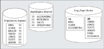
I generally find peoples understanding of what a cluster is in Oracle to be inaccurate. Many people tend to confuse this with a SQL Server or Sybase 'clustered index'. They are not. A cluster is a way to store a group of tables that share some common column(s) in the same database blocks and to store related data together on the same block. A clustered index in SQL Server forces the rows to be stored in sorted order according to the index key, they are similar to an IOT described above. With a cluster, a single block of data may contain data from many tables. Conceptually, you are storing the data 'pre-joined'. It can also be used with single tables. Now you are storing data together grouped by some column. For example, all of the employees in department 10 will be stored on the same block (or as few blocks as possible, if they all don't fit). It is not storing the data sorted - that is the role of the IOT. It is storing the data clustered by some key, but in a heap. So, department 100 might be right next to department 1, and very far away (physically on disk) from departments 101 and 99.
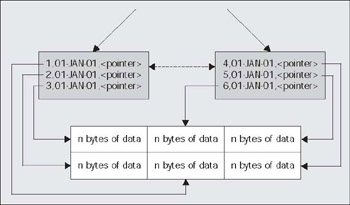
Graphically, you might think of it as I have depicted below. On the left-hand side we are using conventional tables. EMP will be stored in its segment. DEPT will be stored on its own. They may be in different files, different tablespaces, and are definitely in separate extents. On the right-hand side, we see what would happen if we clustered these two tables together. The square boxes represent database blocks. We now have the value 10 factored out and stored once. Then, all of the data from all of the tables in the cluster for department 10 is stored in that block. If all of the data for department 10 does not fit on the block, then additional blocks will be chained to the original block to contain the overflow, very much in the same fashion as the overflow blocks for an IOT:
So, let's look at how you might go about creating a clustered object. Creating a cluster of tables in it is straightforward. The definition of the storage of the object (PCTFREE, PCTUSED, INITIAL, and so on) is associated with the CLUSTER, not the tables. This makes sense since there will be many tables in the cluster, and they each will be on the same block. Having different PCTFREEs would not make sense. Therefore, a CREATECLUSTER looks a lot like a CREATETABLE with a small number of columns (just the cluster key columns):
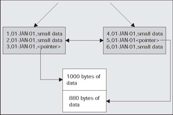
Here we have created an index cluster (the other type being a hash cluster; we'll look at that below). The clustering column for this cluster will be the DEPTNO column, the columns in the tables do not have to be called DEPTNO, but they must be a NUMBER(2), to match this definition. I have, on the cluster definition, a SIZE1024 option. This is used to tell Oracle that we expect about 1,024 bytes of data to be associated with each cluster key value. Oracle will use that to compute the maximum number of cluster keys that could fit per block. Given that I have an 8 KB block size, Oracle will fit up to seven cluster keys (but maybe less if the data is larger then expected) per database block. This is, the data for the departments 10, 20, 30, 40, 50, 60, 70 would tend to go onto one block, as soon as you insert department 80 a new block will be used. That does not mean that the data is stored in a sorted manner, it just means that if you inserted the departments in that order, they would naturally tend to be put together. If you inserted the departments in the following order: 10, 80, 20, 30, 40, 50, 60, and then 70, the final department, 70, would tend to be on the newly added block. As we'll see below, both the size of the data and the order in which the data is inserted will affect the number of keys we can store per block.
The size parameter therefore controls the maximum number of cluster keys per block. It is the single largest influence on the space utilization of your cluster. Set the size too high and you'll get very few keys per block and you'll use more space then you need. Set the size too low and you'll get excessive chaining of data, which offsets the purpose of the cluster to store all of the data together on a single block. It is the important parameter for a cluster.
Now, for the cluster index on our cluster. We need to index the cluster before we can put data in it. We could create tables in the cluster right now, but I am going to create and populate the tables simultaneously and we need a cluster index before we can have any data. The cluster index's job is to take a cluster key value and return the block address of the block that contains that key. It is a primary key in effect where each cluster key value points to a single block in the cluster itself. So, when you ask for the data in department 10, Oracle will read the cluster key, determine the block address for that and then read the data. The cluster key index is created as follows:
tkyte@TKYTE816> create index emp_dept_cluster_idx 2 on cluster emp_dept_cluster 3 /Index created.
It can have all of the normal storage parameters of an index and can be stored in another tablespace. It is just a regular index, one that happens to index into a cluster and can also include an entry for a completely null value (see Chapter 7 on Indexes for the reason why this is interesting to note). Now we are ready to create our tables in the cluster:
Here the only difference from a 'normal' table is that I used the CLUSTER keyword and told Oracle which column of the base table will map to the cluster key in the cluster itself. We can now load them up with the initial set of data:
tkyte@TKYTE816> begin 2 for x in ( select * from scott.dept ) 3 loop 4 insert into dept 5 values ( x.deptno, x.dname, x.loc ); 6 insert into emp 7 select * 8 from scott.emp 9 where deptno = x.deptno; 10 end loop; 11 end; 12 /PL/SQL procedure successfully completed.
You might be asking yourself 'Why didn't we just insert all of the DEPT data and then all of the EMP data or vice-versa, why did we load the data DEPTNO by DEPTNO like that?' The reason is in the design of the cluster. I was simulating a large, initial bulk load of a cluster. If I had loaded all of the DEPT rows first - we definitely would have gotten our 7 keys per block (based on the SIZE1024 setting we made) since the DEPT rows are very small, just a couple of bytes. When it came time to load up the EMP rows, we might have found that some of the departments had many more than 1,024 bytes of data. This would cause excessive chaining on those cluster key blocks. By loading all of the data for a given cluster key at the same time, we pack the blocks as tightly as possible and start a new block when we run out of room. Instead of Oracle putting up to seven cluster key values per block, it will put as many as can fit. A quick example will show the difference between the two approaches. What I will do is add a large column to the EMP table; a CHAR(1000). This column will be used to make the EMP rows much larger then they are now. We will load the cluster tables in two ways - once we'll load up DEPT and then load up EMP. The second time we'll load by department number - a DEPT row and then all the EMP rows that go with it and then the next DEPT. We'll look at the blocks each row ends up on, in the given case, to see which one best achieves the goal of co-locating the data by DEPTNO. In this example, our EMP table looks like:
create table emp( empno number primary key, ename varchar2(10), job varchar2(9), mgr number, hiredate date, sal number, comm number, deptno number(2) references dept(deptno), data char(1000) default '*')cluster emp_dept_cluster(deptno)/
When we load the data into the DEPT and the EMP tables we see that many of the EMP rows are not on the same block as the DEPT row anymore (DBMS_ROWID is a supplied package useful for peeking at the contents of a row ID):
More then half of the EMP rows are not on the block with the DEPT row. Loading the data using the cluster key instead of the table key, we get:
tkyte@TKYTE816> begin 2 for x in ( select * from scott.dept ) 3 loop 4 insert into dept 5 values ( x.deptno, x.dname, x.loc ); 6 insert into emp 7 select emp.*, 'x' 8 from scott.emp 9 where deptno = x.deptno; 10 end loop; 11 end; 12 /PL/SQL procedure successfully completed.tkyte@TKYTE816> select dbms_rowid.rowid_block_number(dept.rowid) dept_rid, 2 dbms_rowid.rowid_block_number(emp.rowid) emp_rid, 3 dept.deptno 4 from emp, dept 5 where emp.deptno = dept.deptno 6 / DEPT_RID EMP_RID DEPTNO---------- ---------- ------ 11 11 30 11 11 30 11 11 30 11 11 30 11 11 30 11 11 30 12 12 10 12 12 10 12 12 10 12 12 20 12 12 20 12 12 20 12 10 20 12 10 2014 rows selected.
Most of the EMP rows are on the same block as the DEPT rows are. This example was somewhat contrived in that I woefully undersized the SIZE parameter on the cluster to make a point, but the approach suggested is correct for an initial load of a cluster. It will ensure that if for some of the cluster keys you exceed the estimated SIZE, you will still end up with most of the data clustered on the same block. If you load a table at a time, you will not.
This only applies to the initial load of a cluster - after that, you would use it as your transactions deem necessary, you will not adapt you application to work specifically with a cluster.
Here is a bit of puzzle to amaze and astound your friends with. Many people mistakenly believe a row ID uniquely identifies a row in a database, that given a row ID I can tell you what table the row came from. In fact, you cannot. You can and will get duplicate row IDs from a cluster. For example, after executing the above you should find:
tkyte@TKYTE816> select rowid from emp 2 intersect 3 select rowid from dept;ROWID------------------AAAGB0AAFAAAAJyAAAAAAGB0AAFAAAAJyAABAAAGB0AAFAAAAJyAACAAAGB0AAFAAAAJyAAD
Every row ID assigned to the rows in DEPT has been assigned to the rows in EMP as well. That is because it takes a table and row ID to uniquely identify a row. The row ID pseudo column is unique only within a table.
I also find that many people believe the cluster object to be an esoteric object that no one really uses. Everyone just uses normal tables. The fact is, that you use clusters every time you use Oracle. Much of the data dictionary is stored in various clusters. For example:
sys@TKYTE816> select cluster_name, table_name from user_tables 2 where cluster_name is not null 3 order by 1 4 /CLUSTER_NAME TABLE_NAME------------------------------ ------------------------------C_COBJ# CCOL$ CDEF$C_FILE#_BLOCK# SEG$ UET$C_MLOG# MLOG$ SLOG$C_OBJ# ATTRCOL$ COL$ COLTYPE$ CLU$ ICOLDEP$ LIBRARY$ LOB$ VIEWTRCOL$ TYPE_MISC$ TAB$ REFCON$ NTAB$ IND$ ICOL$C_OBJ#_INTCOL# HISTGRM$C_RG# RGCHILD$ RGROUP$C_TOID_VERSION# ATTRIBUTE$ COLLECTION$ METHOD$ RESULT$ TYPE$ PARAMETER$C_TS# FET$ TS$C_USER# TSQ$ USER$33 rows selected.
As can be seen, most of the object related data is stored in a single cluster (the C_OBJ# cluster), 14 tables all together sharing the same block. It is mostly column-related information stored there, so all of the information about the set of columns of a table or index is stored physically on the same block. This makes sense; when Oracle parses a query, it wants to have access to the data for all of the columns in the referenced table. If this data was spread all over the place, it would take a while to get it together. Here it is on a single block typically, and readily available.
When would you use a cluster? It is easier perhaps to describe when not to use them:
Clusters may negatively impact the performance of DML - If you anticipate the tables in the cluster to be modified heavily, you must be aware that an index cluster will have certain negative performance side effects. It takes more work to manage the data in a cluster.
Full scans of tables in clusters are affected - Instead of just having to full scan the data in your table, you have to full scan the data for (possibly) many tables. There is more data to scan through. Full scans will take longer.
If you believe you will frequently need to TRUNCATE and load the table - Tables in clusters cannot be truncated, that is obvious since the cluster stores more then one table on a block, we must delete the rows in a cluster table.
So, if you have data that is mostly read (that does not mean 'never written', it is perfectly OK to modify cluster tables) and read via indexes, either the cluster key index or other indexes you put on the tables in the cluster, and join this information together frequently, a cluster would be appropriate. Look for tables that are logically related and always used together, like the people who designed the Oracle data dictionary when they clustered all column-related information together.
Index Clustered Tables Wrap-up
Clustered tables give you the ability to physically 'pre-join' data together. You use clusters to store related data from many tables on the same database block. Clusters can help read intensive operations that always join data together or access related sets of data (for example, everyone in department 10). They will reduce the number of blocks that Oracle must cache; instead of keeping 10 blocks for 10 employees in the same department, they will be put in one block and therefore would increase the efficiency of your buffer cache. On the downside, unless you can calculate your SIZE parameter setting correctly, clusters may be inefficient with their space utilization and can tend to slow down DML heavy operations.
Hash Cluster Tables
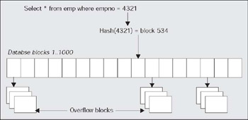
Hash clustered tables are very similar in concept to the index cluster described above with one main exception. The cluster key index is replaced with a hash function. The data in the table is the index, there is no physical index. Oracle will take the key value for a row, hash it using either an internal function or one you supply, and use that to figure out where the data should be on disk. One side effect of using a hashing algorithm to locate data however, is that you cannot range scan a table in a hash cluster without adding a conventional index to the table. In an index cluster above, the query:
select * from emp where deptno between 10 and 20
would be able to make use of the cluster key index to find these rows. In a hash cluster, this query would result in a full table scan unless you had an index on the DEPTNO column. Only exact equality searches may be made on the hash key without using an index that supports range scans.
In a perfect world, with little to no collisions in the hashing algorithm, a hash cluster will mean we can go straight from a query to the data with one I/O. In the real world, there will most likely be collisions and row chaining periodically, meaning we'll need more then one I/O to retrieve some of the data.
Like a hash table in a programming language, hash tables in the database have a fixed 'size'. When you create the table, you must determine the number of hash keys your table will have, forever. That does not limit the amount of rows you can put in there.
Below, we can see a graphical representation of a hash cluster with table EMP created in it. When the client issues a query that uses the hash cluster key in the predicate, Oracle will apply the hash function to determine which block the data should be in. It will then read that one block to find the data. If there have been many collisions or the SIZE parameter to the CREATECLUSTER was underestimated, Oracle will have allocated overflow blocks that are chained off of the original block.
When you create a hash cluster, you will use the same CREATECLUSTER statement you used to create the index cluster with different options. We'll just be adding a HASHKEYs option to it to specify the size of the hash table. Oracle will take your HASHKEYS values and round it up to the nearest prime number, the number of hash keys will always be a prime. Oracle will then compute a value based on the SIZE parameter multiplied by the modified HASHKEYS value. It will then allocate at least that much space in bytes for the cluster. This is a big difference from the index cluster above, which dynamically allocates space, as it needs it. A hash cluster pre-allocates enough space to hold (HASHKEYS/trunc(blocksize/SIZE)) bytes of data. So for example, if you set your SIZE to 1,500 bytes and you have a 4 KB block size, Oracle will expect to store 2 keys per block. If you plan on having 1,000 HASHKEYs, Oracle will allocate 500 blocks.
It is interesting to note that unlike a conventional hash table in a computer language, it is OK to have hash collisions, in fact, it is desirable in many cases. If you take the same DEPT/EMP example from above, you could set up a hash cluster based on the DEPTNO column. Obviously, many rows will hash to the same value - you expect them to (they have the same DEPTNO), this is what the cluster is about in some respects, clustering like data together. This is why Oracle asks you to specify the HASHKEYs (how many department numbers do you anticipate over time) and SIZE (what is the size of the data that will be associated with each department number). It allocates a hash table to hold HASHKEY number of departments of SIZE bytes each. What you do want to avoid is unintended hash collisions. It is obvious that if you set the size of the hash table to 1,000 (really 1,009 since the hash table size is always a prime number and Oracle rounds up for us) and put 1,010 departments in the table, there will be at least one collision (two different departments hashing to the same value). Unintended hash collisions are to be avoided as they add overhead and increase the probability of row chaining occurring.
In order to see what sort of space hash clusters take, we'll write a small utility stored procedure SHOW_SPACE that we'll use in this chapter and in the next chapter on Indexes. This routine just uses the DBMS_SPACE routines we've seen in part above to display space used by objects in the database:
Now if I issue a CREATECLUSTER statement, such as the following, we can see the storage it allocated:
tkyte@TKYTE816> create cluster hash_cluster 2 ( hash_key number ) 3 hashkeys 1000 4 size 8192 5 /Cluster created.tkyte@TKYTE816> exec show_space( 'HASH_CLUSTER', user, 'CLUSTER' )Free Blocks.............................0Total Blocks............................1016Total Bytes.............................8323072Unused Blocks...........................6Unused Bytes............................49152Last Used Ext FileId....................5Last Used Ext BlockId...................889Last Used Block.........................2PL/SQL procedure successfully completed.
I can see that the total number of blocks allocated to the table is 1,016. Six of these blocks are unused (free). One block goes to table overhead, to manage the extents. Therefore, there are 1,009 blocks under the high water mark of this object, and these are used by the cluster. 1,009 just happens to be the next largest prime over 1,000 and since my block size is 8 KB we can see that Oracle did in fact allocate (8192 * 1009) blocks. This figure is a little higher than this, due to the way extents are rounded and/or by using locally managed tablespaces with uniformly-sized extents.
This points out one of the issues with hash clusters you need to be aware of. Normally, if I create an empty table, the number of blocks under the high water mark for that table is 0. If I full scan it, it reaches the high water mark and stops. With a hash cluster, the tables will start out big and will take longer to create as Oracle must initialize each block, an action that normally takes place as data is added to the table. They have the potential to have data in their first block and their last block, with nothing in between. Full scanning a virtually empty hash cluster will take as long as full scanning a full hash cluster. This is not necessarily a bad thing; you built the hash cluster to have very fast access to the data by a hash key lookup. You did not build it to full scan it frequently.
Now I can start placing tables into the hash cluster in the same fashion I did with index clusters. For example:
To see the difference a hash cluster can make, I set up a small test. I created a hash cluster, loaded some data up in it, copied this data to a 'regular' table with a conventional index on it and then I did 100,000 random reads on each table (the same 'random' reads on each). Using SQL_TRACE and TKPROF (more on these tools in Chapter 10 on Tuning Strategies and Tools), I was able to determine the performance characteristics of each. Below is the set up I performed followed by the analysis of it:
I created the hash cluster with a SIZE of 45 bytes. This is because I determined the average row size for a row in my table would be about 45 bytes (I analyzed the SCOTT.EMP table to determine this). I then created an empty table in that cluster that resembles the SCOTT.EMP table. The one modification was to select ROWNUM instead of EMPNO so the table I created was made with a NUMBER instead of NUMBER(4) column. I wanted more than 9,999 rows in this table; I was going for about 50,000. Next I filled up the table and created the 'conventional clone' of it:
tkyte@TKYTE816> declare 2 l_cnt number; 3 l_empno number default 1; 4 begin 5 select count(*) into l_cnt from scott.emp; 6 7 for x in ( select * from scott.emp ) 8 loop 9 for i in 1 .. trunc(50000/l_cnt)+1 10 loop 11 insert into emp values 12 ( l_empno, x.ename, x.job, x.mgr, x.hiredate, x.sal, 13 x.comm, x.deptno ); 14 l_empno := l_empno+1; 15 end loop; 16 end loop; 17 commit; 18 end; 19 /PL/SQL procedure successfully completed.tkyte@TKYTE816> create table emp_reg 2 as 3 select * from emp;Table created.tkyte@TKYTE816> alter table emp_reg add constraint emp_pk primary key(empno);Table altered.
Now, all I needed was some 'random' data to pick rows from each of the tables with:
tkyte@TKYTE816> create table random ( x int );Table created.tkyte@TKYTE816> begin 2 for i in 1 .. 100000 3 loop 4 insert into random values 5 ( mod(abs(dbms_random.random),50000)+1 ); 6 end loop; 7 end; 8 /PL/SQL procedure successfully completed.
Now we are ready to do a test:
tkyte@TKYTE816> alter session set sql_trace=true;Session altered.tkyte@TKYTE816> select count(ename) 2 from emp, random 3 where emp.empno = random.x;COUNT(ENAME)------------ 100000tkyte@TKYTE816> select count(ename) 2 from emp_reg, random 3 where emp_reg.empno = random.x;COUNT(ENAME)------------ 100000
I knew the optimizer would FULLSCAN random in both cases since there is no other access method available for that table. I was counting on it doing a nested loops join to the EMP and EMP_REG table (which it did). This did 100,000 random reads into the two tables. The TKPROF report shows me:
select count(ename) from emp, random where emp.empno = random.xcall count cpu elapsed disk query current rows------- ------ -------- ---------- ----- ---------- ---------- ----------Parse 1 0.00 0.00 0 0 2 0Execute 1 0.00 0.00 0 0 0 0Fetch 2 3.44 3.57 13 177348 4 1------- ------ -------- ---------- ----- ---------- ---------- ----------total 4 3.44 3.57 13 177348 6 1Misses in library cache during parse: 1Optimizer goal: CHOOSEParsing user id: 66Rows Row Source Operation------- --------------------------------------------------- 1 SORT AGGREGATE 100000 NESTED LOOPS 100001 TABLE ACCESS FULL RANDOM 100000 TABLE ACCESS HASH EMP***************************************************************************select count(ename) from emp_reg, random where emp_reg.empno = random.xcall count cpu elapsed disk query current rows------- ------ -------- ---------- ----- ---------- ---------- ----------Parse 1 0.01 0.01 0 1 3 0Execute 1 0.00 0.00 0 0 0 0Fetch 2 1.80 6.26 410 300153 4 1------- ------ -------- ---------- ----- ---------- ---------- ----------total 4 1.81 6.27 410 300154 7 1Misses in library cache during parse: 1Optimizer goal: CHOOSEParsing user id: 66Rows Row Source Operation------- --------------------------------------------------- 1 SORT AGGREGATE 100000 NESTED LOOPS 100001 TABLE ACCESS FULL RANDOM 100000 TABLE ACCESS BY INDEX ROWID EMP_REG 200000 INDEX UNIQUE SCAN (object id 24743)
The points of interest here are:
The hash cluster did significantly less I/O (query column). This is what we had anticipated. The query simply took the random numbers, performed the hash on them, and went to the block. The hash cluster has to do at least one I/O to get the data. The conventional table with an index had to perform index scans followed by a table access by row ID to get the same answer. The indexed table has to do at least two I/Os to get the data.
The hash cluster query took significantly more CPU. This too could be anticipated. The act of performing a hash is very CPU-intensive. The act of performing an index lookup is I/O-intensive.
The hash cluster query had a better elapsed time. This will vary. On my system (a single user laptop for this test; slow disks but I own the CPU), I was not CPU-bound - I was disk-bound. Since I had exclusive access to the CPU, the elapsed time for the hash cluster query was very close to the CPU time. On the other hand, the disks on my laptop were not the fastest. I spent a lot of time waiting for I/O.
This last point is the important one. When working with computers, it is all about resources and their utilization. If you are I/O bound and perform queries that do lots of keyed reads like I did above, a hash cluster may improve performance. If you are already CPU-bound, a hash cluster will possibly decrease performance since it needs more CPU horsepower. This is one of the major reasons why rules of thumb do not work on real world systems - what works for you might not work for others in similar but different conditions.
There is a special case of a hash cluster and that is a 'single table' hash cluster. This is an optimized version of the general hash cluster we've already looked at. It supports only one table in the cluster at a time (you have to DROP the existing table in a single table hash cluster before you can create another). Additionally, if there is a one to one mapping between hash keys and data rows, the access to the rows is somewhat faster as well. These hash clusters are designed for those occasions when you want to access a table by primary key and do not care to cluster other tables with it. If you need fast access to an employee record by EMPNO - a single table hash cluster might be called for. I did the above test on a single table hash cluster as well and found the performance to be even better than just a hash cluster. I went a step further with this example however and took advantage of the fact that Oracle will allow me to write my own specialized hash function (instead of using the default one provided by Oracle). You are limited to using only the columns available in the table and may only use the Oracle built-in functions (no PL/SQL code for example) when writing these hash functions. By taking advantage of the fact that EMPNO is a number between 1 and 50,000 in the above example - I made my 'hash function' simply be the EMPNO column itself. In this fashion, I am guaranteed to never have a hash collision. Putting it all together, we'll create a single table hash cluster with my own hash function via:
tkyte@TKYTE816> create cluster single_table_hash_cluster 2 ( hash_key INT ) 3 hashkeys 50000 4 size 45 5 single table 6 hash is HASH_KEY 7 /Cluster created.
We've simply added the key words SINGLETABLE to make it a single table hash cluster. Our HASHIS function is simply the HASH_KEY cluster key in this case. This is a SQL function, we could have used trunc(mod(hash_key/324+278,555)/abs(hash_key+1))if we wanted (not that this is a good hash function, it just demonstrates that you can use a complex function there if you wish). Then, we create our table in that cluster:
tkyte@TKYTE816> insert into single_table_emp 2 select * from emp;50008 rows created.
After running the same query we did for the other two tables, we discover from the TKPROF report that:
select count(ename) from single_table_emp, random where single_table_emp.empno = random.xcall count cpu elapsed disk query current rows------- ------ -------- ---------- ----- ---------- ---------- ----------Parse 1 0.00 0.00 0 0 0 0Execute 1 0.00 0.00 0 0 0 0Fetch 2 3.29 3.44 127 135406 4 1------- ------ -------- ---------- ----- ---------- ---------- ----------total 4 3.29 3.44 127 135406 4 1Misses in library cache during parse: 0Optimizer goal: CHOOSEParsing user id: 264Rows Row Source Operation------- --------------------------------------------------- 1 SORT AGGREGATE 100000 NESTED LOOPS 100001 TABLE ACCESS FULL RANDOM 100000 TABLE ACCESS HASH SINGLE_TABLE_EMP
This query processed three quarters of the number of blocks that the other hash cluster did. This is due to some combination of using our own hash function that assured us of no collisions and using a single table hash cluster.
Hash Clusters Wrap-up
That is the 'nuts and bolts' of a hash cluster. They are similar in concept to the index cluster above with the exception that a cluster index is not used. The data is the index in this case. The cluster key is hashed into a block address and the data is expected to be there. The important things to really understand are that:
The hash cluster is allocated right from the beginning. Oracle will take your HASHKEYS/trunc(blocksize/SIZE) and will allocate that space right away. As soon as the first table is put in that cluster, any full scan will hit every allocated block. This is different from every other table in this respect.
The number of HASHKEYs in a hash cluster is a fixed size. You cannot change the size of the hash table without a rebuild of the cluster. This does not in any way limit the amount of data you can store in this cluster, it simply limits the number of unique hash keys that can be generated for this cluster. That may affect performance due to unintended hash collisions if it was set too low.
Range scanning on the cluster key is not available. Predicates such as WHEREcluster_keyBETWEEN50AND60 cannot use the hashing algorithm. There are an infinite number of possible values between 50 and 60 - the server would have to generate them all in order to hash each one and see if there was any data there. This is not possible. The cluster will be full scanned if you use a range on a cluster key and have not indexed it using a conventional index.
Hash clusters are suitable when:
You know with a good degree of accuracy how many rows the table will have over its life, or if you have some reasonable upper bound. Getting the size of the HASHKEYs and SIZE parameters right is crucial to avoid a rebuild. If the life of the table is short (for example, a data mart/data warehouse), this is easy.
DML, especially inserts, is light. Updates do not introduce significant overhead, unless you update the HASHKEY, which would not be a good idea. That would cause the row to migrate.
You access the data by the HASHKEY value constantly. For example, you have a table of parts, and part number accesses these parts. Lookup tables are especially appropriate for hash clusters.
Nested Tables
Nested tables are part of the Object Relational Extensions to Oracle. A nested table, one of the two collection types in Oracle, is very similar to a child table in a traditional parent/child table pair in the relational model. It is an unordered set of data elements, all of the same data type, which could either be a built-in data type or an object data type. It goes one step further however, since it is designed to give the illusion that each row in the parent table has its own child table. If there are 100 rows in the parent table, then there are virtually 100 nested tables. Physically, there is only the single parent and the single child table. There are large syntactic and semantic differences between nested tables and parent/child tables as well, and we'll look at those in this section.
There are two ways to use nested tables. One is in your PL/SQL code as a way to extend the PL/SQL language. We cover this technique in Chapter 20 Using Object Relational Features. The other is as a physical storage mechanism, for persistent storage of collections. I personally use them in PL/SQL all of the time but very infrequently as a permanent storage mechanism.
What I am going to do in this section is briefly introduce the syntax to create, query, and modify nested tables. Then we will look at some of the implementation details, what is important to know about how Oracle really stores them.
Nested Tables Syntax
The creation of a table with a nested table is fairly straightforward, it is the syntax for manipulating them that gets a little complex. I will use the simple EMP and DEPT tables to demonstrate. We are familiar with that little data model which is implemented relationally as:
with primary and foreign keys. We will do the equivalent implementation using a nested table for the EMP table:
tkyte@TKYTE816> create or replace type emp_type 2 as object 3 (empno number(4), 4 ename varchar2(10), 5 job varchar2(9), 6 mgr number(4), 7 hiredate date, 8 sal number(7, 2), 9 comm number(7, 2) 10 ); 11 /Type created.tkyte@TKYTE816> create or replace type emp_tab_type 2 as table of emp_type 3 /Type created.
In order to create a table with a nested table, we need a nested table type. The above code creates a complex object type EMP_TYPE and a nested table type of that called EMP_TAB_TYPE. In PL/SQL, this will be treated much like an array would. In SQL, it will cause a physical nested table to be created. Here is the simple CREATETABLE statement that uses it:
tkyte@TKYTE816> create table dept_and_emp 2 (deptno number(2) primary key, 3 dname varchar2(14), 4 loc varchar2(13), 5 emps emp_tab_type 6 ) 7 nested table emps store as emps_nt;Table created.tkyte@TKYTE816> alter table emps_nt add constraint emps_empno_unique 2 unique(empno) 3 /Table altered.
The important part of this create table is the inclusion of the column EMPS of EMP_TAB_TYPE and the corresponding NESTEDTABLEEMPSSTOREASEMPS_NT. This created a real physical table EMPS_NT separate from, and in addition to, the table DEPT_AND_EMP. I added a constraint on the EMPNO column directly on the nested table in order to make the EMPNO unique as it was in our original relational model. I cannot implement our full data model. However, there is the self-referencing constraint:
tkyte@TKYTE816> alter table emps_nt add constraint mgr_fk 2 foreign key(mgr) references emps_nt(empno);alter table emps_nt add constraint mgr_fk*ERROR at line 1:ORA-30730: referential constraint not allowed on nested table column
This will simply not work. Nested tables do not support referential integrity constraints as they cannot reference any other table, even itself. So, we'll just skip that for now. Now, let's populate this table with the existing EMP and DEPT data:
tkyte@TKYTE816> insert into dept_and_emp 2 select dept.*, 3 CAST( multiset( select empno, ename, job, mgr, hiredate, sal, comm 4 from SCOTT.EMP 5 where emp.deptno = dept.deptno ) AS emp_tab_type ) 6 from SCOTT.DEPT 7 /4 rows created.
There are two things to notice here:
Only 'four' rows were created. There are really only four rows in the DEPT_AND_EMP table. The 14 EMP rows don't really exist independently.
The syntax is getting pretty exotic. CAST and MULTISET - syntax most people have never used. You will find lots of exotic syntax when dealing with object relational components in the database. The MULTISET keyword is used to tell Oracle the subquery is expected to return more then one row (subqueries in a SELECT list have previously been limited to returning 1 row). The CAST is used to instruct Oracle to treat the returned set as a collection type - in this case we CAST the MULTISET to be a EMP_TAB_TYPE. CAST is a general purpose routine not limited in use to collections - for example if you wanted to fetch the EMPNO column from EMP as a VARCHAR2(20) instead of a NUMBER(4) type, you may query: selectcast(empnoasVARCHAR2(20))efromemp;
We are now ready to query the data. Let's see what one row might look like:
tkyte@TKYTE816> select deptno, dname, loc, d.emps AS employees 2 from dept_and_emp d 3 where deptno = 10 4 / DEPTNO DNAME LOC EMPLOYEES(EMPNO, ENAME, JOB, M---------- -------------- ------------- ------------------------------ 10 ACCOUNTING NEW YORK EMP_TAB_TYPE(EMP_TYPE(7782, 'CLARK', 'MANAGER', 7839, '09-JUN-81', 2450, NULL), EMP_TYPE(7839, 'KING', 'PRESIDENT', NULL, '17-NOV-81', 5000, NULL), EMP_TYPE(7934, 'MILLER', 'CLERK', 7782, '23-JAN-82', 1300, NULL))
All of the data is there, in a single column. Most applications, unless they are specifically written for the object relational features, will not be able to deal with this particular column. For example, ODBC doesn't have a way to deal with a nested table (JDBC, OCI, Pro*C, PL/SQL, and most other APIs, and languages do). For those cases, Oracle provides a way to un-nest a collection and treats it much like a relational table. For example:
tkyte@TKYTE816> select d.deptno, d.dname, emp.* 2 from dept_and_emp D, table(d.emps) emp 3 /DEPTNO DNAME EMPNO ENAME JOB MGR HIREDATE SAL COMM------ ----------- ----- ---------- --------- ----- --------- ----- ----- 10 ACCOUNTING 7782 CLARK MANAGER 7839 09-JUN-81 2450 10 ACCOUNTING 7839 KING PRESIDENT 17-NOV-81 5000 10 ACCOUNTING 7934 MILLER CLERK 7782 23-JAN-82 1300 20 RESEARCH 7369 SMITH CLERK 7902 17-DEC-80 800 20 RESEARCH 7566 JONES MANAGER 7839 02-APR-81 2975 20 RESEARCH 7788 SCOTT ANALYST 7566 09-DEC-82 3000 20 RESEARCH 7876 ADAMS CLERK 7788 12-JAN-83 1100 20 RESEARCH 7902 FORD ANALYST 7566 03-DEC-81 3000 30 SALES 7499 ALLEN SALESMAN 7698 20-FEB-81 1600 300 30 SALES 7521 WARD SALESMAN 7698 22-FEB-81 1250 500 30 SALES 7654 MARTIN SALESMAN 7698 28-SEP-81 1250 1400 30 SALES 7698 BLAKE MANAGER 7839 01-MAY-81 2850 30 SALES 7844 TURNER SALESMAN 7698 08-SEP-81 1500 0 30 SALES 7900 JAMES CLERK 7698 03-DEC-81 95014 rows selected.
We are able to cast the EMPS column as a table and it naturally did the join for us - no join conditions were needed. In fact, since our EMP type doesn't have the DEPTNO column, there is nothing for us apparently to join on. Oracle takes care of that nuance for us.
So, how can we update the data? Let's say you want to give department 10 a $100 bonus. You would code the following:
tkyte@TKYTE816> update 2 table( select emps 3 from dept_and_emp 4 where deptno = 10 5 ) 6 set comm = 100 7 /3 rows updated.
Here is where the 'virtually a table for every row' comes into play. In the SELECT predicate shown earlier, it may not have been obvious that there was a table per row, especially since the joins and such aren't there, it looks a little like 'magic'. The UPDATE statement however shows that there is a table per row. We selected a discrete table to UPDATE; this table has no name, only a query to identify it. If we use a query that does not SELECTexactly one table, we will receive:
tkyte@TKYTE816> update 2 table( select emps 3 from dept_and_emp 4 where deptno = 1 5 ) 6 set comm = 100 7 /update*ERROR at line 1:ORA-22908: reference to NULL table valuetkyte@TKYTE816> update 2 table( select emps 3 from dept_and_emp 4 where deptno > 1 5 ) 6 set comm = 100 7 / table( select emps *ERROR at line 2:ORA-01427: single-row subquery returns more than one row
If you return less then one row (one nested table instance), the update fails. Normally an update of zero rows is OK but not in this case, it returns an error the same as if you left the table name off of the update. If you return more then one row (more then one nested table instance), the update fails. Normally an update of many rows is perfectly OK. This shows that Oracle considers each row in the DEPT_AND_EMP table to point to another table, not just another set of rows as the relational model does. This is the semantic difference between a nested table and a parent/child relational table. In the nested table model, there is one table per parent row. In the relational model, there is one set of rows per parent row. This difference can make nested tables somewhat cumbersome to use at times. Consider this model we are using, which provides a very nice view of the data from the perspective of single department. It is a terrible model if you want to ask questions like 'what department does KING work for?', 'how many accountants do I have working for me?', and so on. These questions are best asked of the EMP relational table but in this nested table model we can only access the EMP data via the DEPT data. We must always join, we cannot query the EMP data alone. Well, we can't do it in a supported, documented method - we can use a trick (more on this trick later). If we needed to update every row in the EMPS_NT, we would have to do 4 updates; once each for the rows in DEPT_AND_EMP to update the virtual table associated with each row.
Another thing to consider is that when we updated the employee data for department 10, we were semantically updating the EMPS column in the DEPT_AND_EMP table. Physically, we understand there are two tables involved but semantically there is only one. Even though we updated no data in the department table, the row that contains the nested table we did modify is locked from update by other sessions. In a traditional parent/child table relationship, this would not be the case.
These are the reasons why I tend to stay away from nested tables as a persistent storage mechanism. It is the rare child table that is not queried standalone. In the above, the EMP table should be a strong entity. It stands alone, and so, it needs to be queried alone. I find this to be the case almost all of the time. I tend to use nested tables via views on relational tables. We'll investigate this in Chapter 20 on Using Object Relational Features.
So, now that we have seen how to update a nested table instance, inserting and deleting are pretty straightforward. Let's add a row to the nested table instance department 10 and remove a row from department 20:
tkyte@TKYTE816> insert into table 2 ( select emps from dept_and_emp where deptno = 10 ) 3 values 4 ( 1234, 'NewEmp', 'CLERK', 7782, sysdate, 1200, null );1 row created.tkyte@TKYTE816> delete from table 2 ( select emps from dept_and_emp where deptno = 20 ) 3 where ename = 'SCOTT';1 row deleted.tkyte@TKYTE816> select d.dname, e.empno, ename 2 from dept_and_emp d, table(d.emps) e 3 where d.deptno in ( 10, 20 );DNAME EMPNO ENAME-------------- ---------- ----------RESEARCH 7369 SMITHRESEARCH 7566 JONESRESEARCH 7876 ADAMSRESEARCH 7902 FORDACCOUNTING 7782 CLARKACCOUNTING 7839 KINGACCOUNTING 7934 MILLERACCOUNTING 1234 NewEmp8 rows selected.
So, that is the basic syntax of how to query and modify nested tables. You will find many times that you must un-nest these tables as I have above, especially in queries, to make use of them. Once you conceptually visualize the 'virtual table per row' concept, working with nested tables becomes much easier.
Previously I stated: 'We must always join, we cannot query the EMP data alone' but then followed that up with a caveat: 'you can if you really need to'. It is undocumented and not supported, so use it only as a last ditch method. Where it will come in most handy is if you ever need to mass update the nested table (remember, we would have to do that through the DEPT table with a join). There is an undocumented hint, NESTED_TABLE_GET_REFS, used by EXP and IMP to deal with nested tables. It will also be a way to see a little more about the physical structure of the nested tables. This magic hint is easy to discover after you export a table with a nested table. I exported the table above, in order to get its 'larger' definition from IMP. After doing the export, I found the following SQL in my shared pool (V$SQL table):
Well, this is somewhat surprising, if you describe this table:
tkyte@TKYTE816> desc emps_nt Name Null? Type ----------------------------------- -------- ------------------------ EMPNO NUMBER(4) ENAME VARCHAR2(10) JOB VARCHAR2(9) MGR NUMBER(4) HIREDATE DATE SAL NUMBER(7,2) COMM NUMBER(7,2)
These two columns don't even show up. They are part of the hidden implementation of nested tables. The NESTED_TABLE_ID is really a foreign key to the parent table DEPT_AND_EMP. DEPT_AND_EMP which actually has a hidden column in it that is used to join to EMPS_NT. The SYS_NC_ROWINF$ 'column' is a magic column, it is more of a function than a column. The nested table here is really an object table (it is made of an object type) and SYS_NC_INFO$ is the internal way Oracle references the row as an object, instead of referencing each of the scalar columns. Under the covers, all Oracle has done for us is to implement a parent/child table with system generated primary and foreign keys. If we dig a little further, we can query the 'real' data dictionary to see all of the columns in the DEPT_AND_EMP table:
tkyte@TKYTE816> select name 2 from sys.col$ 3 where obj# = ( select object_id 4 from user_objects 5 where object_name = 'DEPT_AND_EMP' ) 6 /NAME------------------------------DEPTNODNAMELOCEMPSSYS_NC0000400005$tkyte@TKYTE816> select SYS_NC0000400005$ from dept_and_emp;SYS_NC0000400005$--------------------------------9A39835005B149859735617476C9A80EA7140089B1954B39B73347EC20190D6820D4AA0839FB49B0975FBDE367842E1656350C866BA24ADE8CF9E47073C52296
The weird looking column name, SYS_NC0000400005$, is the system-generated key placed into the DEPT_AND_EMP table. If you dig even further you will find that Oracle has placed a unique index on this column. Unfortunately however, it neglected to index the NESTED_TABLE_ID in EMPS_NT. This column really needs to be indexed, as we are always joining fromDEPT_AND_EMPtoEMPS_NT. This is an important thing to remember about nested tables if you use them with all of the defaults as I did above, always index the NESTED_TABLE_ID in the nested tables!
I've gotten off of the track though at this point. I was talking about how to treat the nested table as if it were a real table. The NESTED_TABLE_GET_REFS hint does that for us. We can use that like this:
tkyte@TKYTE816> select /*+ nested_table_get_refs */ empno, ename 2 from emps_nt where ename like '%A%'; EMPNO ENAME---------- ---------- 7782 CLARK 7876 ADAMS 7499 ALLEN 7521 WARD 7654 MARTIN 7698 BLAKE 7900 JAMES7 rows selected.tkyte@TKYTE816> update /*+ nested_table_get_refs */ emps_nt 2 set ename = initcap(ename);14 rows updated.tkyte@TKYTE816> select /*+ nested_table_get_refs */ empno, ename 2 from emps_nt where ename like '%a%'; EMPNO ENAME---------- ---------- 7782 Clark 7876 Adams 7521 Ward 7654 Martin 7698 Blake 7900 James6 rows selected.
Again, this is not a documented supported feature. It may not work in all environments. It has a specific functionality - for EXP and IMP to work. This is the only environment it is assured to work in. Use it at your own risk. Use it with caution though, and do not put it into production code. Use it for one-off fixes of data or to see what is in the nested table out of curiosity. The supported way to report on the data is to un-nest it like this:
This is what you should use in queries and production code.
Nested Table Storage
We have already seen some of the storage of the nested table structure. We'll take a more in-depth look at the structure created by Oracle by default, and what sort of control over that we have. Working with the same create statement from above:
tkyte@TKYTE816> create table dept_and_emp 2 (deptno number(2) primary key, 3 dname varchar2(14), 4 loc varchar2(13), 5 emps emp_tab_type 6 ) 7 nested table emps store as emps_nt;Table created.tkyte@TKYTE816> alter table emps_nt add constraint emps_empno_unique 2 unique(empno) 3 /Table altered.
We know that Oracle really creates a structure like this:
The code created two real tables. The table we asked to have is there but it has an extra hidden column (we'll have one extra hidden column by default for each nested table column in a table). It also created a unique constraint on this hidden column. Oracle created the nested table for us - EMPS_NT. This table has two hidden columns, one that is not really a column, SYS_NC_ROWINFO$, but really a virtual column that returns all of the scalar elements as an object. The other is the foreign key, called NESTED_TABLE_ID, which can be joined back to the parent table. Notice the lack of an index on this column! Finally, Oracle added an index on the DEPTNO column in the DEPT_AND_EMP table in order to enforce the primary key. So, we asked for a table and got a lot more then we bargained for. If you look at it, it is a lot like what you might create for a parent/child relationship, but we would have used the existing primary key on DEPTNO as the foreign key in EMPS_NT instead of generating a surrogate RAW(16) key.
If we look at the EXP/IMP dump of our nested table example, we see the following:
CREATE TABLE "TKYTE"."DEPT_AND_EMP"("DEPTNO" NUMBER(2, 0), "DNAME" VARCHAR2(14), "LOC" VARCHAR2(13), "EMPS" "EMP_TAB_TYPE")PCTFREE 10 PCTUSED 40 INITRANS 1 MAXTRANS 255 LOGGINGSTORAGE(INITIAL 131072 NEXT 131072 MINEXTENTS 1 MAXEXTENTS 4096 PCTINCREASE 0 FREELISTS 1 FREELIST GROUPS 1 BUFFER_POOL DEFAULT)TABLESPACE "USERS"NESTED TABLE "EMPS" STORE AS "EMPS_NT" RETURN AS VALUE
The only new thing we notice here so far is the RETURNASVALUE. It is used to describe how the nested table is returned to a client application. By default, Oracle will return the nested table by value to the client - the actual data will be transmitted with each row. This can also be set to RETURNASLOCATOR meaning the client will get a pointer to the data, not the data itself. If, and only if, the client de-references this pointer will the data be transmitted to it. So, if you believe the client will typically not look at the rows of a nested table for each parent row, you can return a locator instead of the values, saving on the network round trips. For example, if you have a client application that displays the lists of departments and when the user double clicks on a department it shows the employee information, you may consider using the locator. This is because the details are usually not looked at - it is the exception, not the rule.
So, what else can we do with the nested table? Firstly, the NESTED_TABLE_ID column must be indexed. Since we always access the nested table from the parent to the child, we really need that index. We can index that column using the create index but a better solution is to use an index organized table to store the nested table. The nested table is another perfect example of what an IOT is excellent for. It will physically store the child rows co-located by NESTED_TABLE_ID (so retrieving the table is done with less physical I/O). It will remove the need for the redundant index on the RAW(16) column. Going one step further, since the NESTED_TABLE_ID will be the leading column in the IOT's primary key, we should also incorporate index key compression to suppress the redundant NESTED_TABLE_ID s that would be there otherwise. In addition, we can incorporate our UNIQUE and NOTNULL constraint on the EMPNO column into the CREATETABLE command. Therefore, if I take the above CREATETABLE and modify it slightly:
CREATE TABLE "TKYTE"."DEPT_AND_EMP"("DEPTNO" NUMBER(2, 0), "DNAME" VARCHAR2(14), "LOC" VARCHAR2(13), "EMPS" "EMP_TAB_TYPE")PCTFREE 10 PCTUSED 40 INITRANS 1 MAXTRANS 255 LOGGINGSTORAGE(INITIAL 131072 NEXT 131072 MINEXTENTS 1 MAXEXTENTS 4096 PCTINCREASE 0 FREELISTS 1 FREELIST GROUPS 1 BUFFER_POOL DEFAULT)TABLESPACE "USERS"NESTED TABLE "EMPS" STORE AS "EMPS_NT" ( (empno NOT NULL, unique (empno), primary key(nested_table_id,empno)) organization index compress 1 ) RETURN AS VALUE/
and now we get the following set of objects. Instead of having a conventional table EMP_NT, we now have an IOT EMPS_NT as signified by the index structure overlaid on the table below:
Where the EMPS_NT is an IOT using compression, this should take less storage than the original default nested table and it has the index we badly need.
Nested Tables Wrap-up
I do not use nested tables as a permanent storage mechanism myself, and this is for the following reasons:
The overhead of the RAW(16) columns that are added. Both the parent and child table will have this extra column. The parent table will have an extra 16 byte RAW for each nested table column it has. Since the parent table typically already has a primary key (DEPTNO in my examples) it would make sense to use this in the child tables, not a system generated key.
The overhead of the unique constraint on the parent table, when it already typically has a unique constraint.
The nested table is not easily used by itself, without using unsupported constructs (NESTED_TABLE_GET_REFS). It can be un-nested for queries but not mass updates.
I do use nested tables heavily as a programming construct and in views. This is where I believe they are in their element and in Chapter 20 on Using Object Relational Features we see how to exploit them in this fashion. As a storage mechanism, I would much prefer creating the parent/child tables myself. After creating the parent/child tables we can in fact create a view that makes it appear as if we had a real nested table. That is, we can achieve all of the advantages of the nested table construct without incurring the overhead. Again in Chapter 20 Using Object Relational Features we'll take a detailed look at how to accomplish this.
If you do use them as a storage mechanism, be sure to make the nested table an index organized table to avoid the overhead of an index on the NESTED_TABLE_ID and the nested table itself. See the section above on IOTs for advice on setting them up with overflow segments and other options. If you do not use an IOT, make sure then to create an index on the NESTED_TABLE_ID column in the nested table to avoid full scanning it to find the child rows.
Temporary Tables
Temporary tables are used to hold intermediate resultsets, either for the duration of a transaction or a session. The data held in a temporary table is only ever visible to the current session - no other session will ever see any other session's data, even if the current session COMMITs the data. Multi-user concurrency is not an issue with regards to temporary tables either, one session can never block another session by using a temporary table. Even if we 'lock' the temporary table, it will not prevent other sessions using their temporary table As we observed in Chapter 3 on Redo and Rollback, temporary tables generate significantly less REDO then regular tables would. However, since they must generate UNDO information for the data they contain, they will generate some amount of REDO Log. UPDATEs and DELETEs will generate the largest amount; INSERTs and SELECTs the least amount.
Temporary tables will allocate storage from the currently logged in users temporary tablespace, or if they are accessed from a definers rights procedure, the temporary tablespace of the owner of that procedure will be used. A global temporary table is really just a template for the table itself. The act of creating a temporary table involves no storage allocation; no INITIAL extent is allocated, as it would be for a non-temporary table. Rather, at runtime when a session first puts data into the temporary table a temporary segment for that session will be created at that time. Since each session gets its own temporary segment, (not just an extent of an existing segment) every user might be allocating space for their temporary table in different tablespaces. USER1 might have their temporary tablespace set to TEMP1 - their temporary tables will be allocated from this space. USER2 might have TEMP2 as their temporary tablespace and their temporary tables will be allocated there.
Oracle's temporary tables are similar to temporary tables in other relational databases with the main exception being that they are 'statically' defined. You create them once per database, not once per stored procedure in the database. They always exist - they will be in the data dictionary as objects, but will always appear empty until your session puts data into them. The fact that they are statically defined allows us to create views that reference temporary tables, to create stored procedures that use static SQL to reference them, and so on.
Temporary tables may be session-based (data survives in the table across commits but not a disconnect/reconnect). They may also be transaction-based (data disappears after a commit). Here is an example showing the behavior of both. I used the SCOTT.EMP table as a template:
tkyte@TKYTE816> create global temporary table temp_table_session 2 on commit preserve rows 3 as 4 select * from scott.emp where 1=0 5 /Table created.
The ONCOMMITPRESERVEROWS clause makes this a session-based temporary table. Rows will stay in this table until my session disconnects or I physically remove them via a DELETE or TRUNCATE. Only my session can see these rows; no other session will ever see 'my' rows even after I COMMIT:
tkyte@TKYTE816> create global temporary table temp_table_transaction 2 on commit delete rows 3 as 4 select * from scott.emp where 1=0 5 /Table created.
The ONCOMMITDELETEROWS makes this a transaction-based temporary table. When your session commits, the rows disappear. The rows will disappear by simply giving back the temporary extents allocated to our table - there is no overhead involved in the automatic clearing of temporary tables. Now, let's look at the differences between the two types:
tkyte@TKYTE816> insert into temp_table_session select * from scott.emp;14 rows created.tkyte@TKYTE816> insert into temp_table_transaction select * from scott.emp;14 rows created.
We've just put 14 rows into each temp table and this shows we can 'see' them:
tkyte@TKYTE816> select session_cnt, transaction_cnt 2 from ( select count(*) session_cnt from temp_table_session ), 3 ( select count(*) transaction_cnt from temp_table_transaction );SESSION_CNT TRANSACTION_CNT----------- --------------- 14 14tkyte@TKYTE816> commit;
Since we've committed, we'll see the session-based rows but not the transaction-based rows:
tkyte@TKYTE816> select session_cnt, transaction_cnt 2 from ( select count(*) session_cnt from temp_table_session ), 3 ( select count(*) transaction_cnt from temp_table_transaction );SESSION_CNT TRANSACTION_CNT----------- --------------- 14 0tkyte@TKYTE816> disconnectDisconnected from Oracle8i Enterprise Edition Release 8.1.6.0.0 - ProductionWith the Partitioning optionJServer Release 8.1.6.0.0 - Productiontkyte@TKYTE816> connect tkyte/tkyteConnected.
Since we've started a new session, we'll see no rows in either table:
tkyte@TKYTE816> select session_cnt, transaction_cnt 2 from ( select count(*) session_cnt from temp_table_session ), 3 ( select count(*) transaction_cnt from temp_table_transaction );SESSION_CNT TRANSACTION_CNT----------- --------------- 0 0
If you have experience of temporary tables in SQL Server and/or Sybase, the major consideration for you is that instead of executing selectx,y,zinto#tempfromsome_table to dynamically create and populate a temporary table, you will:
Once per database, create all of your TEMP tables as a global temporary table. This will be done as part of the application install, just like creating your permanent tables.
In your procedures simply insertintotemp(x,y,z)selectx,y,yfrom some_table.
Just to drive home the point, the goal here is to not create tables in your stored procedures at runtime. That is not the proper way to do this in Oracle. DDL is an expensive operation, we want to avoid doing that at runtime. The temporary tables for an application should be created during the application installation never at run-time.
Temporary tables can have many of the attributes of a permanent table. They may have triggers, check constraints, indexes, and so on. Features of permanent tables that they do not support include:
They cannot have referential integrity constraints - they can neither be the target of a foreign key, nor may they have a foreign key defined on them.
They cannot have VARRAY or NESTEDTABLE type columns.
They cannot be indexed organized tables.
They cannot be in an index or hash cluster.
They cannot be partitioned.
They cannot have statistics generated via the ANALYZE table command.
One of the drawbacks of a temporary table in any database, is the fact that the optimizer has no real statistics on it. When using the Cost-BasedOptimizer (CBO), valid statistics are vital to the optimizer's success (or failure). In the absence of statistics, the optimizer will make guesses as to the distribution of data, the amount of data, the selectivity of an index. When these guesses are wrong, the query plans generated for queries that make heavy use of temporary tables could be less than optimal. In many cases, the correct solution is to not use a temporary table at all, but rather to use an INLINEVIEW (for an example of an INLINEVIEW refer to the last SELECT we ran above - it has two of them) in its place. In this fashion, Oracle will have access to all of the relevant statistics for a table and can come up with an optimal plan.
I find many times people use temporary tables because they learned in other databases that joining too many tables in a single query is a 'bad thing'. This is a practice that must be unlearned for Oracle development. Rather then trying to out-smart the optimizer and breaking what should be a single query into three or four queries that store their sub results into temporary tables and then joining the temporary tables, you should just code a single query that answers the original question. Referencing many tables in a single query is OK; the temporary table crutch is not needed in Oracle for this purpose.
In other cases however, the use of a temporary table in a process is the correct approach. For example, I recently wrote a Palm Sync application to synchronize the date book on a Palm Pilot with calendar information stored in Oracle. The Palm gives me a list of all records that have been modified since the last hot synchronization. I must take these records and compare them against the live data in the database, update the database records and then generate a list of changes to be applied to the Palm. This is a perfect example of when a temporary table is very useful. I used a temporary table to store the changes from the Palm in the database. I then ran a stored procedure that bumps the palm generated changes against the live (and very large) permanent tables to discover what changes need to be made to the Oracle data and then to find the changes that need to come from Oracle back down to the Palm. I have to make a couple of passes on this data, first I find all records that were modified only on the Palm and make the corresponding changes in Oracle. I then find all records that were modified on both the Palm and my database since the last synchronization and rectify them. Then I find all records that were modified only on the database and place their changes into the temporary table. Lastly, the Palm sync application pulls the changes from the temporary table and applies them to the Palm device itself. Upon disconnection, the temporary data goes away.
The issue I encountered however is that because the permanent tables were analyzed, the CBO was being used. The temporary table had no statistics on it (you can analyze the temporary table but no statistics are gathered) and the CBO would 'guess' many things about it. I, as the developer, knew the average number of rows you might expect, the distribution of the data, the selectivity of the indexes and so on. I needed a way to inform the optimizer of these better guesses. The DBMS_STATS package is a great way to do this.
Since the ANALYZE command does not collect statistics on a temporary table, we must use a manual process to populate the data dictionary with representative statistics for our temporary tables. For example, if on average the number of rows in the temporary table will be 500, the average row size will be 100 bytes and the number of blocks will be 7, we could simply use:
Now, the optimizer won't use its best guess, it will use our best guess for this information. Going a step further, we can use Oracle to set the statistics to an even greater level of detail. The following example shows the use of a temporary table with the CBO. The query plan generated without statistics is sub-optimal; the CBO chose to use an index when it should not have. It did that because it assumed default information about index selectivity, number of rows in the table and number of rows to be returned and such. What I did to correct this was to drop the temporary table for a moment, create a permanent table of the same name and structure and populated it with representative data. I then analyzed this table as thoroughly as I wanted to (I could generate histograms and so on as well) and used DBMS_STATS to export the statistics for this permanent table. I then dropped the permanent table and recreated my temporary table. All I needed to do then was import my representative statistics and the optimizer did the right thing:
tkyte@TKYTE816> create global temporary table temp_all_objects 2 as 3 select * from all_objects where 1=0 4 /Table created.tkyte@TKYTE816> create index temp_all_objects_idx on temp_all_objects(object_id) 2 /Index created.tkyte@TKYTE816> insert into temp_all_objects 2 select * from all_objects where rownum < 51 3 /50 rows created.tkyte@TKYTE816> set autotrace on explaintkyte@TKYTE816> select /*+ ALL_ROWS */ object_type, count(*) 2 FROM temp_all_objects 3 where object_id < 50000 4 group by object_type 5 /OBJECT_TYPE COUNT(*)------------------ ----------JAVA CLASS 50Execution Plan---------------------------------------------------------- 0 SELECT STATEMENT Optimizer=HINT: ALL_ROWS (Cost=13 Card=409 1 0 SORT (GROUP BY) (Cost=13 Card=409 Bytes=9816) 2 1 TABLE ACCESS (BY INDEX ROWID) OF 'TEMP_ALL_OBJECTS' (Cost=10 3 2 INDEX (RANGE SCAN) OF 'TEMP_ALL_OBJECTS_IDX' (NON-UNIQUE)tkyte@TKYTE816> set autotrace off
This shows that the CBO did the wrong thing. Any time you access more than 10-20 percent of the table, you should not use an index. Here, we accessed 100 percent of the table; in fact the table is so small that using the index in this case is not buying us anything at all. Here is how to give the optimizer the information it needs to develop the correct plan:
tkyte@TKYTE816> drop table temp_all_objects;Table dropped.tkyte@TKYTE816> create table temp_all_objects 2 as 3 select * from all_objects where 1=0 4 /Table created.tkyte@TKYTE816> create index temp_all_objects_idx on temp_all_objects(object_id) 2 /Index created.tkyte@TKYTE816> insert into temp_all_objects 2 select * from all_objects where rownum < 51;50 rows created.tkyte@TKYTE816> analyze table temp_all_objects compute statistics;Table analyzed.tkyte@TKYTE816> analyze table temp_all_objects compute statistics for all 2 indexes;Table analyzed.
What I have done is created a permanent table that looks just like the temporary table. I populated it with representative data. That is the tricky part here; you must carefully consider what you put into this table when you analyze it. You will be overriding the optimizer's best guess with this data so you had better be giving it better data than it can make up itself. In some cases, it might be enough to just set the table or index statistics manually, as I did above to inform the CBO as the to the cardinality, and range of values. In other cases, you may need to add many pieces of information to the data dictionary in order to give the CBO the data it needs. Instead of manually adding this data, we can let Oracle do the work for us. The method below gets all of the information that you can set easily:
We've just put statistics in our temporary table, based on our representative result set. The CBO will now use this to make decisions about the plans based on that table as evidenced by the next query:
tkyte@TKYTE816> insert into temp_all_objects 2 select * from all_objects where rownum < 51 3 /50 rows created.tkyte@TKYTE816> set autotrace ontkyte@TKYTE816> select /*+ ALL_ROWS */ object_type, count(*) 2 FROM temp_all_objects 3 where object_id < 50000 4 group by object_type 5 /OBJECT_TYPE COUNT(*)------------------ ----------JAVA CLASS 50Execution Plan---------------------------------------------------------- 0 SELECT STATEMENT Optimizer=HINT: ALL_ROWS (Cost=3 Card=1 Bytes=14) 1 0 SORT (GROUP BY) (Cost=3 Card=1 Bytes=14) 2 1 TABLE ACCESS (FULL) OF 'TEMP_ALL_OBJECTS' (Cost=1 Card=50
Temporary Table Wrap-up
Temporary tables can be useful in an application where you need to temporarily store a set of rows to be processed against other tables, either for a session or a transaction. They are not meant to be used as a means to take a single larger query and 'break it up' into smaller result sets that would be joined back together (which seems to be the most popular use of temporary tables in other databases). In fact, you will find in almost all cases that a single query broken up into smaller temporary table queries, performs more slowly in Oracle than the single query would have. I've seen this behavior time and time again, when given the opportunity to write the series of INSERTs into temporary tables as SELECTs in the form of one large query, it goes much faster.
Temporary tables generate a minimum amount of REDO, however, they still generate some REDO and there is no way to disable that. The REDO is generated for the rollback data and in most typical uses will be negligible. If you only INSERT and SELECT from temporary tables, the amount of REDO generated will not be noticeable. Only if you DELETE or UPDATE a temporary table heavily will you see large amounts of redo generated.
Statistics used by the CBO cannot be generated on a temporary table, however, a better guess set of statistics may be set on a temporary table using the DBMS_STATS package. You may either set a few of the relevant statistics such as the number of rows, average row length, and so on, or you may use a permanent table populated with representative data to generate a complete set. One word of caution, make sure your guess is better than the default guess, otherwise the query plans that the CBO generates will be even worse than before.
Object Tables
We have already seen a partial example of an object table above with nested tables. An object table is a table that is created based on a TYPE, not as a collection of columns. Normally, a CREATETABLE would look like this:
create table t ( x int, y date, z varchar2(25);
An object table creation statement looks more like this:
create table t of Some_Type;
The attributes (columns) of t are derived from the definition of SOME_TYPE. Let's look at a quick example involving a couple of types and review the resulting data structures:
tkyte@TKYTE816> create or replace type address_type 2 as object 3 ( city varchar2(30), 4 street varchar2(30), 5 state varchar2(2), 6 zip number 7 ) 8 /Type created.tkyte@TKYTE816> create or replace type person_type 2 as object 3 ( name varchar2(30), 4 dob date, 5 home_address address_type, 6 work_address address_type 7 ) 8 /Type created.tkyte@TKYTE816> create table people of person_type 2 /Table created.tkyte@TKYTE816> desc people Name Null? Type ----------------- -------- ------------ NAME VARCHAR2(30) DOB DATE HOME_ADDRESS ADDRESS_TYPE WORK_ADDRESS ADDRESS_TYPE
So, in a nutshell that's all there is to it. You create some type definitions and then you can create tables of that type. The table appears to have four columns representing the four attributes of the PERSON_TYPE we created. We are at the point where we can now perform DML on the object table to create and query data:
tkyte@TKYTE816> insert into people values ( 'Tom', '15-mar-1965', 2 address_type( 'Reston', '123 Main Street', 'Va', '45678' ), 3 address_type( 'Redwood', '1 Oracle Way', 'Ca', '23456' ) );1 row created.tkyte@TKYTE816> select * from people;NAME DOB HOME_ADDRESS(CITY, S WORK_ADDRESS(CI---- --------- -------------------- ---------------Tom 15-MAR-65 ADDRESS_TYPE('Reston ADDRESS_TYPE('R ', '123 Main edwood', '1 Street', 'Va', Oracle Way', 45678) 'Ca', 23456)tkyte@TKYTE816> select name, p.home_address.city from people p;NAME HOME_ADDRESS.CITY---- ------------------------------Tom Reston
You are starting to see some of the object syntax necessary to deal with object types. For example, in the INSERT statement we had to wrap the HOME_ADDRESS and WORK_ADDRESS with a CAST. We cast the scalar values to be of an ADDRESS_TYPE. Another way of saying this is that we create an ADDRESS_TYPE instance for that row by using the default constructor for the ADDRESS_TYPE object.
Now, as far as the external face of the table is concerned, there are four columns in our table. By now, after seeing the hidden magic that took place for the nested tables, we can probably guess that there is something else going on. Oracle stores all object relational data in plain old relational tables - at the end of the day it is all in rows and columns. If we dig into the 'real' data dictionary, we can see what this table really looks like:
This looks quite different from what describe tells us. Apparently, there are 14 columns in this table, not 4. In this case they are:
SYS_NC_OID$ - This is the system-generated object ID of the table. It is a unique RAW(16) column. It has a unique constraint on it - there is a corresponding unique index created on it as well.
SYS_NC_ROWINFO - This is the same 'magic' function as we observed with the nested table. If we select that from the table it returns the entire row as a single column.:
NAME, DOB - These are the scalar attributes of our object table. They are stored much as you would expect, as regular columns
HOME_ADDRESS, WORK_ADDRESS - These are 'magic' functions as well, they return the collection of columns they represent as a single object. These consume no real space except to signify NULL or NOTNULL for the entity.
SYS_NCnnnnn$ - These are the scalar implementations of our embedded object types. Since the PERSON_TYPE had the ADDRESS_TYPE embedded in it, Oracle needed to make room to store them in the appropriate type of columns. The system-generated names are necessary since a column name must be unique and there is nothing stopping us from using the same object type more then once as we did here. If the names were not generated, we would have ended up with the ZIP column twice.
So, just like with the nested table, there is lots going on here. A pseudo primary key of 16 bytes was added, there are virtual columns, and an index created for us. We can change the default behavior with regards to the value of the object identifier assigned to an object, as we'll see in a moment. First, let's look at the full verbose SQL that would generate our table for us, again this was generated using EXP/IMP:
This gives us a little more insight into what is actually taking place here. We see the OIDINDEX clause clearly now and we see a reference to the SYS_NC_OID$ column. This is the hidden primary key of the table. The function SYS_OP_GUID, is the same as the function SYS_GUID. They both return a globally unique identifier that is a 16 byte RAW field.
The OID'<bighexnumber>' syntax is not documented in the Oracle documentation. All this is doing is ensuring that during an EXP and subsequent IMP, the underlying type PERSON_TYPE is in fact the same type. This will prevent an error that would occur if you:
Created the PEOPLE table.
Exported it.
Dropped it and the underlying PERSON_TYPE.
Created a new PERSON_TYPE with different attributes.
Imported the old PEOPLE data.
Obviously, this export cannot be imported into the new structure - it will not fit. This check prevents that from occurring. You can refer to the Chapter 8 on Import and Export later on for guidelines regarding import and export and more details on object tables.
If you remember, I mentioned that we can change the behavior of the object identifier assigned to an object instance. Instead of having the system generate a pseudo primary key for us, we can use the natural key of an object. At first, this might appear self defeating - the SYS_NC_OID$ will still appear in the table definition in SYS.COL$, and in fact it, will appear to consume massive amounts of storage as compared to the system generated column. Once again however, there is 'magic' at work here. The SYS_NC_OID$ column for an object table that is based on a primarykey and not system generated, is a virtual column and consumes no real storage on disk. Here is an example that shows what happens in the data dictionary and shows that there is no physical storage consume for the SYS_NC_OID$. We'll start with an analysis of the system generated OID table:
tkyte@TKYTE816> CREATE TABLE "TKYTE"."PEOPLE" 2 OF "PERSON_TYPE" 3 /Table created.tkyte@TKYTE816> select name, type#, segcollength 2 from sys.col$ 3 where obj# = ( select object_id 4 from user_objects 5 where object_name = 'PEOPLE' ) 6 and name like 'SYS\_NC\_%' escape '\' 7 /NAME TYPE# SEGCOLLENGTH------------------------------ ---------- ------------SYS_NC_OID$ 23 16SYS_NC_ROWINFO$ 121 1tkyte@TKYTE816> insert into people(name) 2 select rownum from all_objects;21765 rows created.tkyte@TKYTE816> analyze table people compute statistics;Table analyzed.tkyte@TKYTE816> select table_name, avg_row_len from user_object_tables;TABLE_NAME AVG_ROW_LEN------------------------------ -----------PEOPLE 25
So, we see here that the average row length is 25 bytes, 16 bytes for the SYS_NC_OID$ and 9 bytes for the NAME. Now, let's do the same thing, but use a primary key on the NAME column as the object identifier:
tkyte@TKYTE816> CREATE TABLE "TKYTE"."PEOPLE" 2 OF "PERSON_TYPE" 3 ( constraint people_pk primary key(name) ) 4 object identifier is PRIMARY KEY 5 /Table created.tkyte@TKYTE816> select name, type#, segcollength 2 from sys.col$ 3 where obj# = ( select object_id 4 from user_objects 5 where object_name = 'PEOPLE' ) 6 and name like 'SYS\_NC\_%' escape '\' 7 /NAME TYPE# SEGCOLLENGTH------------------------------ ---------- ------------SYS_NC_OID$ 23 81SYS_NC_ROWINFO$ 121 1
According to this, instead of a small 16 byte column, we have a large 81 byte column! In reality, there is no data stored in there. It will be Null. The system will generate a unique ID based on the object table, its underlying type and the value in the row itself. We can see this in the following:
tkyte@TKYTE816> insert into people (name) 2 values ( 'Hello World!' );1 row created.tkyte@TKYTE816> select sys_nc_oid$ from people p;SYS_NC_OID$------------------------------------------------------------7129B0A94D3B49258CAC926D8FDD6EEB00000017260100010001002900000000000C07001E0100002A00078401FE000000140C48656C6C6F20576F726C6421000000000000000000000000000000000000tkyte@TKYTE816> select utl_raw.cast_to_raw( 'Hello World!' ) data 2 from dual;DATA------------------------------------------------------------48656C6C6F20576F726C6421tkyte@TKYTE816> select utl_raw.cast_to_varchar2(sys_nc_oid$) data 2 from people;DATA------------------------------------------------------------<garbage data .>Hello World!
If we select out the SYS_NC_OID$ column and inspect the HEX dump of the string we inserted, we see that the row data itself is embedded in the object ID. Converting the object id into a VARCHAR2, we can just confirm that visually. Does that mean our data is stored twice with a lot of overhead with it? Actually it can not:
tkyte@TKYTE816> insert into people(name) 2 select rownum from all_objects;21766 rows created.tkyte@TKYTE816> analyze table people compute statistics;Table analyzed.tkyte@TKYTE816> select table_name, avg_row_len from user_object_tables;TABLE_NAME AVG_ROW_LEN------------------------------ -----------PEOPLE 8
The average row length is only 8 bytes now. The overhead of storing the system-generated key is gone and the 81 bytes you might think we are going to have isn't really there. Oracle synthesizes the data upon selecting from the table.
Now for an opinion. The object relational components (nested tables, object tables) are primarily what I call 'syntactic sugar'. They are always translated into 'good old' relational rows and columns. I prefer not to use them as physical storage mechanisms personally. There are too many bits of 'magic' happening - side effects that are not clear. You get hidden columns, extra indexes, surprise pseudo columns, and so on. This does not mean that the object relational components are a waste of time, on the contrary really. I use them in PL/SQL constantly. I use them with object views. I can achieve the benefits of a nested table construct (less data returned over the network for a master detail relationship, conceptually easier to work with, and so on) without any of the physical storage concerns. That is because I can use object views to synthesize my objects from my relational data. This solves most all of my concerns with object tables/nested tables in that the physical storage is dictated by me, the join conditions are setup by me, and the tables are available as relational tables (which is what many third party tools and applications will demand) naturally. The people who require an object view of relational data can have it and the people who need the relational view have it. Since object tables are really relational tables in disguise, we are doing the same thing Oracle does for us behind the scenes, only we can do it more efficiently, since we don't have to do it generically as they do. For example, using the types defined above I could just as easily use the following:
tkyte@TKYTE816> create table people_tab 2 ( name varchar2(30) primary key, 3 dob date, 4 home_city varchar2(30), 5 home_street varchar2(30), 6 home_state varchar2(2), 7 home_zip number, 8 work_city varchar2(30), 9 work_street varchar2(30), 10 work_state varchar2(2), 11 work_zip number 12 ) 13 /Table created.tkyte@TKYTE816> create view people of person_type 2 with object identifier (name) 3 as 4 select name, dob, 5 address_type(home_city,home_street,home_state,home_zip) home_adress, 6 address_type(work_city,work_street,work_state,work_zip) work_adress 7 from people_tab 8 /View created.tkyte@TKYTE816> insert into people values ( 'Tom', '15-mar-1965', 2 address_type( 'Reston', '123 Main Street', 'Va', '45678' ), 3 address_type( 'Redwood', '1 Oracle Way', 'Ca', '23456' ) );1 row created.
However I achieve very much the same effect, I know exactly what is stored, how it is stored, and where it is stored. For more complex objects we may have to code INSTEADOF triggers on the Object Views to allow for modifications through the view.
Object Table Wrap-up
Object tables are used to implement an object relational model in Oracle. A single object table will create many physical database objects typically, and add additional columns to your schema to manage everything. There is some amount of 'magic' associated with object tables. Object Views allow you to take advantage of the syntax and semantics of 'objects' while at the same time retaining complete control over the physical storage of the data and allowing for relational access to the underlying data. In that fashion, you can achieve the best of both the relational and object relational worlds.
Summary
Hopefully, after reading this chapter you have come to the conclusion that not all tables are created equal. Oracle provides a rich variety of table types that you can exploit. In this chapter, we have covered many of the salient aspects of tables in general and the many different table types Oracle provides for us to use.
We began by looking at some terminology and storage parameters associated with tables. We looked at the usefulness of FREELISTs in a multi-user environment where a table is frequently inserted/updated by many people simultaneously. We investigated the meaning of PCTFREE and PCTUSED, and developed some guidelines for setting them correctly.
Then we got into the different types of tables starting with the common heap. The heap organized table is by far the most commonly used table in most Oracle applications and is the default table type. We moved onto index organized tables, the ability store your table data in an index. We saw how these are applicable for various uses such as lookup tables and inverted lists where a heap table would just be a redundant copy of the data. Later, we saw how they can really be useful when mixed with other table types, specifically the nested table type.
We looked at cluster objects of which Oracle has two kinds; Index and Hash. The goals of the cluster are twofold:
To give us the ability to store data from many tables together - on the same database block(s); and
To give us the ability to force like data to be stored physically 'together' based on some cluster key - in this fashion all of the data for department 10 (from many tables) may be stored together.
These features allow us to access this related data very quickly, with minimal physical I/O that might otherwise be needed to pull together all of the data. We observed the main differences between index clusters and hash clusters and discussed when each would be appropriate (and when they would not).
Next, we moved onto Nested Tables. We reviewed the syntax, semantics, and usage of these types of tables. We saw how they are in a fact a system generated and maintained parent/child pair of tables and discovered how Oracle physically does this for us. We looked at using different table types for Nested tables which by default use a heap based table. We found that there would probably never be a reason not to use an IOT instead of a heap table for nested tables.
Then we looked into the ins and outs of Temporary tables; looking at how to create them, where they get their storage from, and the fact that they introduce no concurrency related issues at runtime. We explored the differences between session level and transaction level temporary table. We discussed the appropriate method for using temporary tables in an Oracle database.
This section closed up with a look into the workings of object tables. Like nested tables, we discovered there is a lot going on under the covers with object tables in Oracle. We discussed how object views on top of relational tables can give us the functionality of an object table while at the same time giving us access to the underlying relational data easily; a topic we will look at in more detail in Chapter 20 on Using Object Relational Features.