Indexing is a crucial aspect of your application design and development. Too many indexes and the performance of DML will suffer. Too few indexes and the performance of queries (including inserts, updates and deletes) will suffer. Finding the right mix is critical to your application performance.
I find frequently that indexes are an afterthought in application development. I believe that this is the wrong approach. From the very beginning, if you understand how the data will be used, you should be able to come up with the representative set of indexes you will use in your application. Too many times the approach seems to be to throw the application out there and then see where indexes are needed. This implies you have not taken the time to understand how the data will be used and how many rows you will ultimately be dealing with. You'll be adding indexes to this system forever as the volume of data grows over time (reactive tuning). You'll have indexes that are redundant, never used, and this wastes not only space but also computing resources. A few hours at the start, spent properly considering when and how to index your data will save you many hours of 'tuning' further down the road (note that I said 'it will', not 'it might').
The basic remit of this chapter is to give an overview of the indexes available for use in Oracle and discuss when and where you might use them. This chapter will differ from others in this book in terms of its style and format. Indexing is a huge topic - you could write an entire book on the subject. Part of the reason for this is that it bridges the developer and DBA roles. The developer must be aware of them, how they apply to their applications, when to use them (and when not to use them), and so on. The DBA is concerned with the growth of an index, the degree of fragmentation within an index and other physical properties. We will be tackling indexes mainly from the standpoint of their practical use in applications (we will not deal specifically with index fragmentation, and so on). The first half of this chapter represents the basic knowledge I believe you need in order to make intelligent choices about when to index and what type of index to use. The second answers some of the most frequently asked questions about indexes.
The various examples in this book require different base releases of Oracle. When a specific feature requires Oracle 8i Enterprise or Personal Edition I'll specify that. Many of the B*Tree indexing examples require Oracle 7.0 and later versions. The bitmap indexing examples require Oracle 7.3.3 or later versions (Enterprise or Personal edition). Function-based indexes and application domain indexes require Oracle 8i Enterprise or Personal Editions. The section Frequently Asked Questions applies to all releases of Oracle.
An Overview of Oracle Indexes
Oracle provides many different types of indexes for us to use. Briefly they are as follows:
B*Tree Indexes - These are what I refer to as 'conventional' indexes. They are by far the most common indexes in use in Oracle, and most other databases. Similar in construct to a binary tree, they provide fast access, by key, to an individual row or range of rows, normally requiring few reads to find the correct row. The B*Tree index has several 'subtypes':
Index Organized Tables - A table stored in a B*Tree structure. We discussed these in some detail Chapter 4, Tables. That section also covered the physical storage of B*Tree structures, so we will not cover that again here.
B*Tree Cluster Indexes - These are a slight variation of the above index. They are used to index the cluster keys (see Index Clustered Tables in Chapter 4) and will not be discussed again in this chapter. They are used not to go from a key to a row, but rather from a cluster key to the block that contains the rows related to that cluster key.
Reverse Key Indexes - These are B*Tree indexes where the bytes in the key are 'reversed'. This is used to more evenly distribute index entries throughout an index that is populated with increasing values. For example, if I am using a sequence to generate a primary key, the sequence will generate values like 987500, 987501, 987502, and so on. Since these values are sequential, they would all tend to go the same block in the index, increasing contention for that block. With a reverse key index, Oracle would be indexing: 205789, 105789, 005789 instead. These values will tend to be 'far away' from each other in the index and would spread out the inserts into the index over many blocks.
Descending Indexes - In the future, descending indexes will not be notable as a special type of index. However, since they are brand new with Oracle 8i they deserve a special look. Descending indexes allow for data to be sorted from 'big' to 'small' (descending) instead of small to big (ascending) in the index structure. We'll take a look at why that might be important and how they work.
Bitmap Indexes - Normally in a B*Tree, there is a one-to-one relationship between an index entry and a row - an index entry points to a row. With a bitmap index, a single index entry uses a bitmap to point to many rows simultaneously. They are appropriate for low cardinality data (data with few distinct values) that is mostly read-only. A column that takes on three values: Y, N, and NULL, in a table of one million rows might be a good candidate for a bitmap index. Bitmap indexes should never be considered in an OLTP database for concurrency related issues (which we'll discuss in due course).
Function-based indexes - These are B*Tree or Bitmap indexes that store the computed result of a function on a rows column(s) - not the column data itself. These may be used to speed up queries of the form: SELECT*FROMTWHERE FUNCTION(DATABASE_COLUMN)=SOME_VALUE since the value FUNCTION(DATABASE_COLUMN) has already been computed and stored in the index.
Application Domain Indexes - These are indexes you build and store yourself, either in Oracle or perhaps even outside of Oracle. You will tell the optimizer how selective your index is, how costly it is to execute and the optimizer will decide whether or not to use your index, based on that information. The interMedia text index is an example of an application domain index; it is built using the same tools you may use to build your own index.
interMedia Text Indexes - This is a specialized index built into Oracle to allow for keyword searching of large bodies of text. We'll defer a discussion of these until the Chapter 17 on interMedia.
As you can see, there are many types of indexes to choose from. What I would like to do in the following sections is to present some technical details on how they work and when they should be used. I would like to stress again that we will not be covering certain DBA-related topics. For example, we will not cover the mechanics of an online rebuild, but rather will concentrate on practical application-related details.
B*Tree Indexes
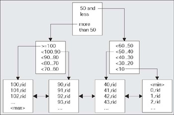
B*Tree, or what I call 'conventional', indexes are the most commonly used type of indexing structure in the database. They are similar in implementation to a binary search tree. Their goal is to minimize the amount of time Oracle spends searching for data. Loosely speaking, if you have an index on a number column then the structure might look like this:
The lowest level blocks in the tree, called leafnodes, contain every indexed key and a row ID (rid in the picture) that points to the row it is indexing. The interior blocks, above the leaf nodes, are known as branch blocks. They are used to navigate through the structure. For example, if we wanted to find the value 42 in the index, we would start at the top of the tree and go to the right. We would inspect that block and discover we needed to go to the block in the range 'less than 50 to 40'. This block would be the leaf block and would point us to the rows that contained the number 42. It is interesting to note that the leaf nodes of the index are actually a doubly linked list. Once we find out where to 'start' in the leaf nodes - once we have found that first value- doing an ordered scan of values (also known as an index range scan) is very easy. We don't have to navigate the structure any more; we just go forward through the leaf nodes. That makes solving a predicate, such as the following, pretty simple:
where x between 20 and 30
Oracle finds the first index block that contains 20 and then just walks horizontally, through the linked list of leaf nodes until, it finally hits a value that is greater than 30.
There really is no such thing as a non-unique index in a B*Tree. In a non-unique index, Oracle simply adds the row's row ID to the index key to make it unique. In a unique index, as defined by you, Oracle does not add the row ID to the index key. In a non-unique index, we will find that the data is sorted first by index key values (in the order of the index key), and then by row ID. In a unique index, the data is sorted by the index key values only.
One of the properties of a B*Tree is that all leaf blocks should be at the same level in the tree, although technically, the difference in height across the tree may vary by one. This level is also known as the height of the index, meaning that all the nodes above the leaf nodes only point to lower, more specific nodes, while entries in the leaf nodes point to specific row IDs, or a range of row IDs. Most B*Tree indexes will have a height of 2 or 3, even for millions of records. This means that it will take, in general, 2 or 3 reads to find your key in the index - which is not too bad. Another property is that the leaves, are self-balanced, in other words, all are at the same level, and this is mostly true. There are some opportunities for the index to have less than perfect balance, due to updates and deletes. Oracle will try to keep every block in the index from about three-quarters to completely full although, again, DELETEs and UPDATEs can skew this as well. In general, the B*Tree is an excellent general purpose indexing mechanism that works well for large and small tables and experiences little, if any, degradation as the size of the underlying table grows, as long as the tree does not get skewed.
One of the interesting things you can do with a B*Tree index is to 'compress' it. This is not compression in the same manner that zip files are compressed; rather this is compression that removes redundancies from concatenated indexes. We covered this in some detail in the section Index Organized Tables in Chapter 6, but we will take a brief look at it again here. The basic concept behind a key compressed index is that every entry is broken into two pieces - a 'prefix' and 'suffix' component. The prefix is built on the leading columns of the concatenated index and would have many repeating values. The suffix is the trailing columns in the index key and is the unique component of the index entry within the prefix. For example, we'll create a table and index and measure it's space without compression - then, we'll recreate the index with index key compression enabled and see the difference:
Note
This example calls on the show_space procedure given in Chapter 6 on Tables
tkyte@TKYTE816> create table t 2 as 3 select * from all_objects 4 /Table created.tkyte@TKYTE816> create index t_idx on 2 t(owner,object_type,object_name);Index created.tkyte@TKYTE816>tkyte@TKYTE816> exec show_space('T_IDX',user,'INDEX')Free Blocks.............................0Total Blocks............................192Total Bytes.............................1572864Unused Blocks...........................35Unused Bytes............................286720Last Used Ext FileId....................6Last Used Ext BlockId...................649Last Used Block.........................29PL/SQL procedure successfully completed.
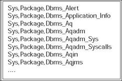
The index allocated 192 blocks and has 35 that contain no data (157 blocks in total use). We could realize that the OWNER component is repeated many times. A single index block will have dozens of entries like this:
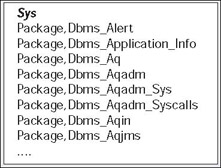
We could factor the repeated OWNER column out of this, resulting in a block that looks more like this:
Here the owner name appears once on the leaf blocks - not once per repeated entry. If we recreate that index using compression with the leading column:
tkyte@TKYTE816> drop index t_idx;Index dropped.tkyte@TKYTE816> create index t_idx on 2 t(owner,object_type,object_name) 3 compress 1;Index created.tkyte@TKYTE816> exec show_space('T_IDX',user,'INDEX')Free Blocks.............................0Total Blocks............................192Total Bytes.............................1572864Unused Blocks...........................52Unused Bytes............................425984Last Used Ext FileId....................6Last Used Ext BlockId...................649Last Used Block.........................12PL/SQL procedure successfully completed.
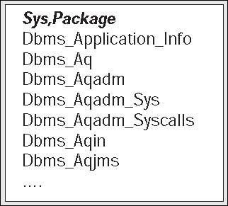
We can see this reduced the size of the overall index structure from 157 used blocks to 140, a reduction of about 10 percent. We can go further, compressing the leading two columns. This will result in blocks where both the OWNER and the OBJECT_TYPE are factored out to the block level:
Now, when we use compression on the leading two columns:
tkyte@TKYTE816> drop index t_idx;Index dropped.tkyte@TKYTE816> create index t_idx on 2 t(owner,object_type,object_name) 3 compress 2;Index created.tkyte@TKYTE816>tkyte@TKYTE816> exec show_space('T_IDX',user,'INDEX')Free Blocks.............................0Total Blocks............................128Total Bytes.............................1048576Unused Blocks...........................15Unused Bytes............................122880Last Used Ext FileId....................6Last Used Ext BlockId...................585Last Used Block.........................49PL/SQL procedure successfully completed.
This index is 113 blocks, about thirty percent smaller then the original index. Depending on how repetitious your data is, this could really add up. Now, you do not get this compression for free. The compressed index structure is now more complex then it used to be. Oracle will spend more time processing the data in this structure, both while maintaining the index during modifications as well as when you search the index during a query. What we are doing here is trading off increased CPU time for reduced I/O time. Our block buffer cache will be able to hold more index entries than before, our cache-hit ratio might go up, our physical I/Os should go down but it will take a little more CPU horse power to process the index and also increases the chance of block contention. Just as in our discussion of the hash cluster, where it took more CPU to retrieve a million random rows but half the I/O, we must be aware of the trade-off. If you are currently CPU-bound, adding compressed key indexes may slow down your processing. On the other hand, if you are I/O bound, using them may speed things up.
Reverse Key Indexes
Another feature of a B*Tree index is the ability to 'reverse' their keys. At first, you might ask yourself, 'Why would I want to do that?' They were designed for a specific environment, for a specific issue. They were implemented to reduce contention on index leaf blocks in an Oracle Parallel Server (OPS) environment.
Note
We discussed OPS in Chapter 2, Architecture.
It is a configuration of Oracle where multiple instances can mount and open the same database. If two instances need to modify the same block of data simultaneously, they will share the block by flushing it to disk so that the other instance can read it. This activity is known as 'pinging'. Pinging is something to be avoided when using OPS but will be virtually unavoidable if you have a conventional B*Tree index, this is on a column whose values are generated by a sequence number. Everyone will be trying to modify the left hand side of the index structure as they insert new values (see the figure at start of the section on B*Tree Indexes that shows 'higher values' in the index go to the left, lower values to the right). In an OPS environment, modifications to indexes on columns populated by sequences are focused on a small set of leaf blocks. Reversing the keys of the index allows insertions to be distributed across all the leaf keys in the index, though it tends to make the index much less efficiently packed.
A reverse key index will simply reverse the bytes of each column in an index key. If we consider the numbers 90101, 90102, 90103,and look at their internal representation using the Oracle DUMP function, we will find they are represented as:
tkyte@TKYTE816> select 90101, dump(90101,16) from dual 2 union all 3 select 90102, dump(90102,16) from dual 4 union all 5 select 90103, dump(90103,16) from dual 6 / 90101 DUMP(90101,16)---------- --------------------- 90101 Typ=2 Len=4: c3,a,2,2 90102 Typ=2 Len=4: c3,a,2,3 90103 Typ=2 Len=4: c3,a,2,4
Each one is four bytes in length and only the last byte is different. These numbers would end up right next to each other in an index structure. If we reverse their bytes however, Oracle will insert:
tkyte@TKYTE816> select 90101, dump(reverse(90101),16) from dual 2 union all 3 select 90102, dump(reverse(90102),16) from dual 4 union all 5 select 90103, dump(reverse(90103),16) from dual 6 / 90101 DUMP(REVERSE(90101),1---------- --------------------- 90101 Typ=2 Len=4: 2,2,a,c3 90102 Typ=2 Len=4: 3,2,a,c3 90103 Typ=2 Len=4: 4,2,a,c3
The numbers will end up 'far away' from each other. This reduces the number of instances going after the same block (the leftmost block) and reduces the amount of pinging going on. One of the drawbacks to a reverse key index is that you cannot utilize it in all of the cases where a regular index can be applied. For example, in answering the following predicate, a reverse key index on x would not be useful:
where x > 5
The data in the index is not sorted before it is stored, hence the range scan will not work. On the other hand, some range scans can be done on a reverse key index. If I have a concatenated index on X, Y, the following predicate will be able to make use of the reverse key index and will 'range scan' it:
where x = 5
This is because the bytes for X are reversed and then the bytes for Y are reversed. Oracle does not reverse the bytes of X||Y, but rather stores reverse(X)||reverse(Y). This means all of the values for X=5 will be stored together, so Oracle can range scan that index to find them all.
Descending Indexes
Descending Indexes are a new feature of Oracle 8i that extend the functionality of a B*Tree index. They allow for a column to be stored sorted from 'big' to 'small' in the index instead of ascending. Prior releases of Oracle have always supported the DESC (descending) keyword, but basically ignored it - it had no effect on how the data was stored or used in the index. In Oracle 8i however, it changes the way the index is created and used.
Oracle has had the ability to read an index backwards for quite a while, so you may be wondering why this feature is relevant. For example, if we used the table T from above and queried:
tkyte@TKYTE816> select owner, object_type 2 from t 3 where owner between 'T' and 'Z' 4 and object_type is not null 5 order by owner DESC, object_type DESC 6 /46 rows selected.Execution Plan---------------------------------------------------------- 0 SELECT STATEMENT Optimizer=CHOOSE (Cost=2 Card=46 Bytes=644) 1 0 INDEX (RANGE SCAN DESCENDING) OF 'T_IDX' (NON-UNIQUE)...
It is shown that Oracle will just read the index backwards, there is no final sort step in this plan, the data is sorted. Where this descending index feature comes into play however, is when you have a mixture of columns and some are sorted ASC (ascending) and some DESC (descending). For example:
tkyte@TKYTE816> select owner, object_type 2 from t 3 where owner between 'T' and 'Z' 4 and object_type is not null 5 order by owner DESC, object_type ASC 6 /46 rows selected.Execution Plan---------------------------------------------------------- 0 SELECT STATEMENT Optimizer=CHOOSE (Cost=4 Card=46 Bytes=644) 1 0 SORT (ORDER BY) (Cost=4 Card=46 Bytes=644) 2 1 INDEX (RANGE SCAN) OF 'T_IDX' (NON-UNIQUE) (Cost=2 Card=
Oracle isn't able to use the index we have in place on (OWNER, OBJECT_TYPE, OBJECT_NAME) anymore to sort the data. It could have read it backwards to get the data sorted by OWNERDESC but it needs to read it 'forwards' to get OBJECT_TYPE sorted ASC. Instead, it collected together all of the rows and then sorted. Enter the DESC index:
tkyte@TKYTE816> create index desc_t_idx on t(owner DESC, object_type ASC ) 2 /Index created.tkyte@TKYTE816> select owner, object_type 2 from t 3 where owner between 'T' and 'Z' 4 and object_type is not null 5 order by owner DESC, object_type ASC 6 /46 rows selected.Execution Plan---------------------------------------------------------- 0 SELECT STATEMENT Optimizer=CHOOSE (Cost=4 Card=46 Bytes=644) 1 0 INDEX (RANGE SCAN) OF 'DESC_T_IDX' (NON-UNIQUE)...
Now, once more, we are able to read the data sorted, there is no extra sort step at the end of the plan. It should be noted that unless your compatibleinit.ora parameter is set to 8.1.0 or higher, the DESC option on the create index will be silently ignored - no warning or error will be produced as this was the default behavior in prior releases.
When should you use a B*Tree Index?
Not being a big believer in 'rules of thumb' (there are exceptions to every rule), I don't have any rules of thumb for when to use (or not to use) a B*Tree index. To demonstrate why I don't have any rules of thumb for this case, I'll present two equally valid ones:
Only use B*Tree to index columns if you are going to access a very small percentage of the rows in the table via the index
Use a B*Tree index if you are going to process many rows of a table and the index can be used insteadof the table.
These rules seem to offer conflicting advice, but in reality, they do not - they just cover two extremely different cases. There are two ways to use an index:
As the means to access rows in a table. You will read the index to get to a row in the table. Here you want to access a very small percentage of the rows in the table.
As the means to answer a query. The index contains enough information to answer the entire query - we will not have to go to the table at all. The index will be used as a 'thinner' version of the table.
The first case above says if you have a table T (using the same table T from above) and you have a query plan looks like this:
tkyte@TKYTE816> set autotrace traceonly explaintkyte@TKYTE816> select owner, status 2 from T 3 where owner = USER;Execution Plan---------------------------------------------------------- 0 SELECT STATEMENT Optimizer=CHOOSE 1 0 TABLE ACCESS (BY INDEX ROWID) OF 'T' 2 1 INDEX (RANGE SCAN) OF 'T_IDX' (NON-UNIQUE)
You should be accessing a very small percentage of this table. The issue to look at here is the INDEX (RANGESCAN) followed by the TABLEACCESSBYINDEXROWID. What this means is that Oracle will read the index and then, for each index entry, it will perform a database block read (logical or physical I/O) to get the row data. This is not the most efficient method if you are going to have to access a large percentage of the rows in T via the index (below we will define what a large percentage might be).
On the other hand, if the index can be used instead of the table, you can process 100 percent (or any percentage in fact) of the rows via the index. This is rule of thumb number two. You might use an index just to create a 'thinner' version of a table (in sorted order to boot).
The following query demonstrates this concept:
tkyte@TKYTE816> select count(*) 2 from T 3 where owner = USER;Execution Plan---------------------------------------------------------- 0 SELECT STATEMENT Optimizer=CHOOSE 1 0 SORT (AGGREGATE) 2 1 INDEX (RANGE SCAN) OF 'T_IDX' (NON-UNIQUE)
Here, only the index was used to answer the query - it would not matter now what percentage of rows we were accessing, we used the index only. We can see from the plan that the underlying table was never accessed; we simply scanned the index structure itself.
It is important to understand the difference between the two concepts. When we have to do a TABLEACCESSBYINDEXROWID, we must ensure we are accessing only a small percentage of the total rows in the table. If we access too high a percentage of the rows (larger then somewhere between 1 and 20 percent of the rows), it will take longer than just full scanning the table. With the second type of query above, where the answer is found entirely in the index, we have a different story. We read an index block and pick up many 'rows' to process, we then go onto the next index block, and so on - we never go to the table. There is also a fast full scan we can perform on indexes to make this even faster in certain cases. A fast full scan is when the database reads the index blocks in no particular order - it just starts reading them. It is no longer using the index as an index, but even more like a table at that point. Rows do not come out ordered by index entries from a fast full scan.
In general, a B*Tree index would be placed on columns that I use frequently in the predicate of a query, and expect some small fraction of the data from the table to be returned. On a 'thin' table, a table with few or small columns, this fraction may be very small. A query that uses this index should expect to retrieve 2 to 3 percent or less of the rows to be accessed in the table. On a 'fat' table, a table with many columns or a table with very wide columns, this fraction might go all of the way up to 20-25 percent of the table. This advice doesn't always seem to make sense to everyone immediately; it is not intuitive, but it is accurate. An index is stored sorted by index key. The index will be accessed in sorted order by key. The blocks that are pointed to are stored randomly in a heap. Therefore, as we read through an index to access the table, we will perform lots of scattered, random I/O. By scattered, I mean that the index will tell us to read block 1, block 1000, block 205, block 321, block 1, block 1032, block 1, and so on - it won't ask us to read block 1, then 2, then 3 in a consecutive manner. We will tend to read and re-read blocks in a very haphazard fashion. Doing this, single block I/O can be very slow.
As a simplistic example of this, let's say we are reading that 'thin' table via an index and we are going to read 20 percent of the rows. Assume we have 100,000 rows in the table. Twenty percent of that is 20,000 rows. If the rows are about 80 bytes apiece in size, on a database with an 8 KB block size, we will find about 100 rows per block. That means the table has approximately 1000 blocks. From here, the math is very easy. We are going to read 20,000 rows via the index; this will mean 20,000 TABLEACCESSBYROWID operations. We will process 20,000 table blocks in order to execute this query. There are only about 1000 blocks in the entire table however! We would end up reading and processing each block in the table on average 20 times! Even if we increased the size of the row by an order of magnitude to 800 bytes per row, 10 rows per block, we now have 10,000 blocks in the table. Index accesses for 20,000 rows would cause us to still read each block on average two times. In this case, a full table scan will be much more efficient than using an index, as it only has to touch each block once. Any query that used this index to access the data, would not be very efficient until it accesses on average less then 5 percent of the data for the 800 byte column (then we access about 5000 blocks) and even less for the 80 byte column (about 0.5 percent or less).
Of course, there are factors that change these calculations. Suppose you have a table where the rows have a primary key populated by a sequence. As data is added to the table, rows with sequential sequence numbers are in general 'next' to each other. The table is naturally clustered, in order, by the primary key, (since the data is added in more or less that order). It will not be strictly clustered in order by the key of course (we would have to use an IOT to achieve that), but in general rows with primary keys that are close in value will be 'close' together in physical proximity. Now when you issue the query:
select * from T where primary_key between :x and :y
The rows you want are typically located on the same blocks. In this case an index range scan may be useful even if it accesses a large percentage of rows, simply because the database blocks that we need to read and re-read will most likely be cached, since the data is co-located. On the other hand, if the rows are not co-located, using that same index may be disastrous for performance. A small demonstration will drive this fact home. We'll start with a table that is pretty much ordered by its primary key:
tkyte@TKYTE816> create table colocated ( x int, y varchar2(2000) ) pctfree 0;Table created.tkyte@TKYTE816> begin 2 for i in 1 .. 100000 3 loop 4 insert into colocated values ( i, rpad(dbms_random.random,75,'*') ); 5 end loop; 6 end; 7 /PL/SQL procedure successfully completed.tkyte@TKYTE816> alter table colocated 2 add constraint colocated_pk primary key(x);Table altered.
This is a table fitting the description we laid out above - about 100 rows/block in my 8 KB database. In this table there is a very good chance that the rows with x=1, 2, 3 are on the same block. Now, we'll take this table and purposely 'disorganize' it. In the COLOCATED table above, we created the Y column with a leading random number - we'll use that fact to 'disorganize' the data - so it will definitely not be ordered by primary key anymore:
tkyte@TKYTE816> create table disorganized nologging pctfree 0 2 as 3 select x, y from colocated ORDER BY y 4 /Table created.tkyte@TKYTE816> alter table disorganized 2 add constraint disorganized_pk primary key(x);Table altered.
Arguably, these are the same tables - it is a relational database, physical organization plays no bearing on how things work (at least that's what they teach in theoretical database courses). In fact, the performance characteristics of these two tables are different as 'night and day'. Given the same exact query:
tkyte@TKYTE816> select * from COLOCATED where x between 20000 and 40000;20001 rows selected.Elapsed: 00:00:01.02Execution Plan---------------------------------------------------------- 0 SELECT STATEMENT Optimizer=CHOOSE 1 0 TABLE ACCESS (BY INDEX ROWID) OF 'COLOCATED' 2 1 INDEX (RANGE SCAN) OF 'COLOCATED_PK' (UNIQUE)Statistics---------------------------------------------------------- 0 recursive calls 0 db block gets 2909 consistent gets 258 physical reads 0 redo size 1991367 bytes sent via SQL*Net to client 148387 bytes received via SQL*Net from client 1335 SQL*Net roundtrips to/from client 0 sorts (memory) 0 sorts (disk) 20001 rows processedtkyte@TKYTE816> select * from DISORGANIZED where x between 20000 and 40000;20001 rows selected.Elapsed: 00:00:23.34Execution Plan---------------------------------------------------------- 0 SELECT STATEMENT Optimizer=CHOOSE 1 0 TABLE ACCESS (BY INDEX ROWID) OF 'DISORGANIZED' 2 1 INDEX (RANGE SCAN) OF 'DISORGANIZED_PK' (UNIQUE)Statistics---------------------------------------------------------- 0 recursive calls 0 db block gets 21361 consistent gets 1684 physical reads 0 redo size 1991367 bytes sent via SQL*Net to client 148387 bytes received via SQL*Net from client 1335 SQL*Net roundtrips to/from client 0 sorts (memory) 0 sorts (disk) 20001 rows processed
I think this is pretty incredible. What a difference physical data layout can make! To summarize the results:
Table
Elapsed Time
Logical I/O
Colocated
1.02 seconds
2,909
Disorganized
23.34 seconds
21,361
In my database using an 8 KB block size - these tables had 1,088 total blocks apiece. The query against disorganized table bears out the simple math we did above - we did 20,000 plus logical I/Os. We processed each and every block 20 times!! On the other hand, the physically COLOCATED data took the logical I/Os way down. Here is the perfect example of why rules of thumb are so hard to provide - in one case, using the index works great, in the other - it stinks. Consider this the next time you dump data from your production system and load it into development - it may very well be part of the answer to the question that typically comes up of 'why is it running differently on this machine - they are identical?' They are not identical.
Just to wrap up this example - let's look at what happens when we full scan the disorganized table:
tkyte@TKYTE816> select /*+ FULL(DISORGANIZED) */ * 2 from DISORGANIZED 3 where x between 20000 and 40000;20001 rows selected.Elapsed: 00:00:01.42Execution Plan---------------------------------------------------------- 0 SELECT STATEMENT Optimizer=CHOOSE (Cost=162 Card=218 Bytes=2 1 0 TABLE ACCESS (FULL) OF 'DISORGANIZED' (Cost=162 Card=218 BStatistics---------------------------------------------------------- 0 recursive calls 15 db block gets 2385 consistent gets 404 physical reads 0 redo size 1991367 bytes sent via SQL*Net to client 148387 bytes received via SQL*Net from client 1335 SQL*Net roundtrips to/from client 0 sorts (memory) 0 sorts (disk) 20001 rows processed
That shows that in this particular case - due to the way the data is physically stored on disk, the full scan is very appropriate. This begs the question - so how can I accommodate for this? The answer is - use the cost based optimizer (CBO) and it will do it for you. The above case so far has been executed in RULE mode since we never gathered any statistics. The only time we used the cost based optimizer was when we hinted the full table scan above and asked the cost based optimizer to do something specific for us. If we analyze the tables, we can take a peek at some of the information Oracle will use to optimize the above queries:
tkyte@TKYTE816> analyze table colocated 2 compute statistics 3 for table 4 for all indexes 5 for all indexed columns 6 /Table analyzed.tkyte@TKYTE816> analyze table disorganized 2 compute statistics 3 for table 4 for all indexes 5 for all indexed columns 6 /Table analyzed.
Now, we'll look at some of the information Oracle will use. We are specifically going to look at the CLUSTERING_FACTOR column found in the USER_INDEXES view. The Oracle Reference Manual tells us this column has the following meaning, it:
Indicates the amount of order of the rows in the table based on the values of the index:
If the value is near the number of blocks, then the table is very well ordered. In this case, the index entries in a single leaf block tend to point to rows in the same data blocks.
If the value is near the number of rows, then the table is very randomly ordered. In this case, it is unlikely that index entries in the same leaf block point to rows in the same data blocks.
The CLUSTERING_FACTOR is an indication of how ordered the table is with respect to the index itself, when we look at these indexes we find:
tkyte@TKYTE816> select a.index_name, 2 b.num_rows, 3 b.blocks, 4 a.clustering_factor 5 from user_indexes a, user_tables b 6 where index_name in ('COLOCATED_PK', 'DISORGANIZED_PK' ) 7 and a.table_name = b.table_name 8 /INDEX_NAME NUM_ROWS BLOCKS CLUSTERING_FACTOR------------------------------ ---------- ---------- -----------------COLOCATED_PK 100000 1063 1063DISORGANIZED_PK 100000 1064 99908
The COLOCATED_PK is a classic 'the table is well ordered' example, whereas the DISORGANIZE_PK is the classic 'the table is very randomly ordered' example. It is interesting to see how this affects the optimizer now. If we attempted to retrieve 20,000 rows, Oracle will now choose a full table scan for both queries (retrieving 20 percent of the rows via an index is not the optimal plan even for the very ordered table). However, if we drop down to 10 percent of the table data:
tkyte@TKYTE816> select * from COLOCATED where x between 20000 and 30000;10001 rows selected.Elapsed: 00:00:00.11Execution Plan---------------------------------------------------------- 0 SELECT STATEMENT Optimizer=CHOOSE (Cost=129 Card=9996 Bytes=839664) 1 0 TABLE ACCESS (BY INDEX ROWID) OF 'COLOCATED' (Cost=129 Card=9996 2 1 INDEX (RANGE SCAN) OF 'COLOCATED_PK' (UNIQUE) (Cost=22 Card=9996)Statistics---------------------------------------------------------- 0 recursive calls 0 db block gets 1478 consistent gets 107 physical reads 0 redo size 996087 bytes sent via SQL*Net to client 74350 bytes received via SQL*Net from client 668 SQL*Net roundtrips to/from client 1 sorts (memory) 0 sorts (disk) 10001 rows processedtkyte@TKYTE816> select * from DISORGANIZED where x between 20000 and 30000;10001 rows selected.Elapsed: 00:00:00.42Execution Plan---------------------------------------------------------- 0 SELECT STATEMENT Optimizer=CHOOSE (Cost=162 Card=9996 Bytes=839664) 1 0 TABLE ACCESS (FULL) OF 'DISORGANIZED' (Cost=162 Card=9996Statistics---------------------------------------------------------- 0 recursive calls 15 db block gets 1725 consistent gets 707 physical reads 0 redo size 996087 bytes sent via SQL*Net to client 74350 bytes received via SQL*Net from client 668 SQL*Net roundtrips to/from client 1 sorts (memory) 0 sorts (disk) 10001 rows processed
Here we have the same table structures - same indexes, but different clustering factors. The optimizer in this case chose an index access plan for the COLOCATED table and a full scan access plan for the DISORGANIZED table.
The key point to this discussion is that indexes are not always the appropriate access method. The optimizer may very well be correct in choosing to not use an index, as the above example demonstrates. There are many factors that influence the use of an index by the optimizer - including physical data layout. You might run out and try to rebuild all of your tables now to make all indexes have a good clustering factor but that most likely would be a waste of time in most cases. It will affect cases where you do index range scans of a large percentage of a table - not a common case in my experience. Additionally, you must keep in mind that in general the table will only have one index with a good clustering factor! The data can only be sorted in one way. In the above example - if I had another index on the column Y - it would be very poorly clustered in the COLOCATED table, but very nicely clustered in the DISORGANIZED table. If having the data physically clustered is important to you - consider the use of an IOT over a table rebuild.
B*Trees Wrap-up
B*Tree indexes are by far the most common and well-understood indexing structures in the Oracle database. They are an excellent general purpose indexing mechanism. They provide very scalable access times, returning data from a 1,000 row index in about the same amount of time as a 100,000 row index structure.
When to index, and what columns to index, is something you need to pay attention to in your design. An index does not always mean faster access; in fact, you will find that indexes will decrease performance in many cases if Oracle uses them. It is purely a function of how large of a percentage of the table you will need to access via the index and how the data happens to be laid out. If you can use the index to 'answer the question', accessing a large percentage of the rows makes sense, since you are avoiding the extra scattered I/O to read the table. If you use the index to access the table, you will need to ensure you are processing a small percentage of the total table.
You should consider the design and implementation of indexes during the design of your application, not as an afterthought (as I so often see). With careful planning and due consideration of how you are going to access the data, the indexes you need will be apparent in most all cases.
Bitmap Indexes
Bitmap Indexes were added to Oracle in version 7.3 of the database. They are currently available with the Oracle 8i Enterprise and Personal Editions, but not the Standard Edition. Bitmap indexes are designed for data warehousing/ad-hoc query environments where the full set of queries that may be asked of the data is not totally known at system implementation time. They are specifically not designed for OLTP systems or systems where data is frequently updated by many concurrent sessions.
Bitmap indexes are structures that store pointers to many rows with a single index key entry, as compared to a B*Tree structure where there is parity between the index keys and the rows in a table. In a bitmap index, there will be a very small number of index entries, each of which point to many rows. In a B*Tree, it is one-to-one - an index entry points to a single row.
Let's say you were creating a bitmap index on the JOB column in the EMP table as follows:
scott@TKYTE816> create BITMAP index job_idx on emp(job);Index created.
Oracle will store something like the following in the index:
Value/Row
1
2
3
4
5
6
7
8
9
10
11
12
13
14
ANALYST
0
0
0
0
0
0
0
1
0
1
0
0
1
0
CLERK
1
0
0
0
0
0
0
0
0
0
1
1
0
1
MANAGER
0
0
0
1
0
1
1
0
0
0
0
0
0
0
PRESIDENT
0
0
0
0
0
0
0
0
1
0
0
0
0
0
SALESMAN
0
1
1
0
1
0
0
0
0
0
0
0
0
0
This shows that rows 8, 10, and 13 have the value ANALYST whereas the rows 4, 6, and 7 have the value MANAGER. It also shows me that no rows are null (Bitmap indexes store null entries - the lack of a null entry in the index implies there are no null rows). If I wanted to count the rows that have the value MANAGER, the bitmap index would do this very rapidly. If I wanted to find all the rows such that the JOB was CLERK or MANAGER, I could simply combine their bitmaps from the index as follows:
Value/Row
1
2
3
4
5
6
7
8
9
10
11
12
13
14
CLERK
1
0
0
0
0
0
0
0
0
0
1
1
0
1
MANAGER
0
0
0
1
0
1
1
0
0
0
0
0
0
0
CLERK or MANAGER
1
0
0
1
0
1
1
0
0
0
1
1
0
1
This rapidly shows me that rows 1, 4, 6, 7, 11, 12, and 14 satisfy my criteria. The bitmap Oracle stores with each key value is set up so that each position represents a row ID in the underlying table, if we need to actually retrieve the row for further processing. Queries such as:
select count(*) from emp where job = 'CLERK' or job = 'MANAGER'
will be answered directly from the bitmap index. A query such as:
select * from emp where job = 'CLERK' or job = 'MANAGER'
on the other hand will need to get to the table. Here Oracle will apply a function to turn the fact that the i'th bit is on in a bitmap, into a row ID that can be used to access the table.
When Should you use a Bitmap Index?
Bitmap indexes are most appropriate on low cardinality data. This is data where the number of distinct items in the set of rows divided by the number of rows is a small number (near zero). For example, a GENDER column might take on the values M, F, and NULL. If you have a table with 20000 employee records in it then you would find that 3/20000 = 0.00015. This column would be a candidate for a bitmap index. It would definitely not be a candidate for a B*Tree index as each of the values would tend to retrieve an extremely large percentage of the table. B*Tree indexes should be selective in general as outlined above. Bitmap indexes should not be selective, on the contrary they should be very 'unselective'.
Bitmap indexes are extremely useful in environments where you have lots of ad-hoc queries, especially queries that reference many columns in an ad-hoc fashion or produce aggregations such as COUNT. For example, suppose you have a table with three columns GENDER, LOCATION, and AGE_GROUP. In this table GENDER has a value of M or F, and LOCATION can take on the values 1 through 50 and AGE_GROUP is a code representing 18andunder, 19-25, 26-30, 31-40, 41and over. You have to support a large number of ad-hoc queries that take the form:
Select count(*) from T where gender = 'M' and location in ( 1, 10, 30 ) and age_group = '41 and over';select * from t where ( ( gender = 'M' and location = 20 ) or ( gender = 'F' and location = 22 )) and age_group = '18 and under';select count(*) from t where location in (11,20,30);select count(*) from t where age_group = '41 and over' and gender = 'F';
You would find that a conventional B*Tree indexing scheme would fail you. If you wanted to use an index to get the answer, you would need at least three and up to six combinations of possible B*Tree indexes in order to access the data. Since any of the three columns or any subset of the three columns may appear, you would need large concatenated B*Tree indexes on:
GENDER, LOCATION, AGE_GROUP - For queries that used all three, or GENDER with LOCATION, or GENDER alone.
LOCATION, AGE_GROUP - For queries that used LOCATION and AGE_GROUP or LOCATION alone.
AGE_GROUP, GENDER - For queries that used AGE_GROUP with GENDER or AGE_GROUP alone.
In order to reduce the amount of data being searched, other permutations might be reasonable as well, to reduce the size of the index structure being scanned. This is ignoring the fact that a B*Tree index on such low cardinality data is not a good idea.
Here the bitmap index comes into play. With three small bitmap indexes, one on each of the individual columns, you will be able to satisfy all of the above predicates efficiently. Oracle will simply use the functions AND, OR, and XOR with the bitmaps of the three indexes together, to find the solution set for any predicate that references any set of these three columns. It will take the resulting merged bitmap, convert the 1s into row IDs if necessary, and access the data (if we are just counting rows that match the criteria, Oracle will just count the 1 bits).
There are times when bitmaps are not appropriate as well. They work well in a read intensive environment, but they are extremely ill-suited for a write intensive environment. The reason is that a single bitmap index key entry points to many rows. If a session modifies the indexed data, then all of the rows that index entry points to are effectively locked. Oracle cannot lock an individual bit in a bitmap index entry; it locks the entire bitmap. Any other modifications that need to update that same bitmap will be locked out. This will seriously inhibit concurrency - each update will appear to lock potentially hundreds of rows preventing their bitmap columns from being concurrently updated. It will not lock every row as you might think, just many of them. Bitmaps are stored in chunks, using the EMP example from above we might find that the index key ANALYST appears in the index many times, each time pointing to hundreds of rows. An update to a row that modifies the JOB column will need to get exclusive access to two of these index key entries; the index key entry for the old value and the index key entry for the new value. The hundreds of rows these two entries point to, will be unavailable for modification by other sessions until that UPDATE commits.
Bitmap Indexes Wrap-up
'When in doubt - try it out'. It is trivial to add a bitmap index to a table (or a bunch of them) and see what they do for you. Also you can usually create bitmap indexes much faster than B*Tree indexes. Experimentation is the best way to see if they are suited for your environment. I am frequently asked 'What defines low cardinality?' There is no cut-and-dry answer for this. Sometimes it is 3 values out of 100,000. Sometimes it is 10,000 values out of 1,000,000. Low cardinality doesn't imply single digit counts of distinct values. Experimentation will be the way to discover if a bitmap is a good idea for your application. In general, if you have a large, mostly read-only environment with lots of ad-hoc queries, a set of bitmap indexes may be exactly what you need.
Function-Based Indexes
Function-based indexes were added to Oracle 8.1.5 of the database. They are currently available with the Oracle8i Enterprise and Personal Editions, but not the Standard Edition.
Function-based indexes give us the ability to index computed columns and use these indexes in a query. In a nutshell, this capability allows you to have case insensitive searches or sorts, search on complex equations, and extend the SQL language efficiently by implementing your own functions and operators and then searching on them.
There are many reasons why you would want to use a function-based index. Leading among them are:
They are easy to implement and provide immediate value.
They can be used to speed up existing applications without changing any of their logic or queries.
Important Implementation Details
In order to make use of function-based Indexes, we must perform some setup work. Unlike B*Tree and Bitmap indexes above, function-based indexes require some initial setup before we can create and then use them. There are some init.ora or session settings you must use and to be able to create them, a privilege you must have. The following is a list of what needs to be done to use function-based indexes:
You must have the system privilege QUERYREWRITE to create function-based indexes on tables in your own schema.
You must have the system privilege GLOBALQUERYREWRITE to create function-based indexes on tables in other schemas.
Use the Cost Based Optimizer. Function-based indexes are only visible to the Cost Based Optimizer and will not be used by the Rule Based Optimizer ever.
Use SUBSTR to constrain return values from user written functions that return VARCHAR2 or RAW types. Optionally hide the SUBSTR in a view (recommended). See below for examples of this.
For the optimizer to use function-based indexes, the following session or system variables must be set:
You may enable these at either the session level with ALTERSESSION, or at the system level via ALTERSYSTEM, or by setting them in the init.ora parameter file. The meaning of QUERY_REWRITE_ENABLED is to allow the optimizer to rewrite the query to use the function-based index. The meaning of QUERY_REWRITE_INTEGRITY is to tell the optimizer to 'trust' that the code marked deterministic by the programmer is in fact deterministic (see below for examples of deterministic code and its meaning). If the code is in fact not deterministic (that is, it returns different output given the same inputs), the resulting rows retrieve via the index may be incorrect. That is something you must take care to ensure.
Once the above list has been satisfied, function-based indexes are as easy to use as the CREATEINDEX command. The optimizer will find and use your indexes at runtime for you.
Function-Based Index Example
Consider the following example. We want to perform a case insensitive search on the ENAME column of the EMP table. Prior to function-based indexes, we would have approached this in a very different manner. We would have added an extra column to the EMP table - called UPPER_ENAME, for example. This column would have been maintained by a database trigger on INSERT and UPDATE - that trigger would simply have set : NEW.UPPER_NAME:=UPPER(:NEW.ENAME). This extra column would have been indexed. Now with function-based indexes, we remove the need for the extra column.
We'll begin by creating a copy of the demo EMP table in the SCOTT schema and add lots of data to it.
tkyte@TKYTE816> create table emp 2 as 3 select * from scott.emp;Table created.tkyte@TKYTE816> set timing ontkyte@TKYTE816> insert into emp 2 select -rownum EMPNO, 3 substr(object_name,1,10) ENAME, 4 substr(object_type,1,9) JOB, 5 -rownum MGR, 6 created hiredate, 7 rownum SAL, 8 rownum COMM, 9 (mod(rownum,4)+1)*10 DEPTNO 10 from all_objects 11 where rownum < 10000 12 /9999 rows created.Elapsed: 00:00:01.02tkyte@TKYTE816> set timing offtkyte@TKYTE816> commit;Commit complete.
Now, we will change the data in the employee name column to be in mixed case. Then we will create an index on the UPPER of the ENAME column, effectively creating a case insensitive index:
tkyte@TKYTE816> update emp set ename = initcap(ename);10013 rows updated.tkyte@TKYTE816> create index emp_upper_idx on emp(upper(ename));Index created.
Finally, we'll analyze the table since, as noted above, we need to make use of the cost based optimizer in order to utilize function-based indexes:
tkyte@TKYTE816> analyze table emp compute statistics 2 for table 3 for all indexed columns 4 for all indexes;Table analyzed.
We now have an index on the UPPER of a column. Any application that already issues 'case insensitive' queries (and has the requisite SYSTEM or SESSION settings), like this:
tkyte@TKYTE816> alter session set QUERY_REWRITE_ENABLED=TRUE;Session altered.tkyte@TKYTE816> alter session set QUERY_REWRITE_INTEGRITY=TRUSTED;Session altered.tkyte@TKYTE816> set autotrace on explaintkyte@TKYTE816> select ename, empno, sal from emp where upper(ename)='KING';ENAME EMPNO SAL---------- ---------- ----------King 7839 5000Execution Plan---------------------------------------------------------- 0 SELECT STATEMENT Optimizer=CHOOSE (Cost=2 Card=9 Bytes=297) 1 0 TABLE ACCESS (BY INDEX ROWID) OF 'EMP' (Cost=2 Card=9 Bytes=297) 2 1 INDEX (RANGE SCAN) OF 'EMP_UPPER_IDX' (NON-UNIQUE) (Cost=1 Card=9)
will make use of this index, gaining the performance boost an index can deliver. Before this feature was available, every row in the EMP table would have been scanned, uppercased, and compared. In contrast, with the index on UPPER(ENAME), the query takes the constant KING to the index, range scans a little data and accesses the table by row ID to get the data. This is very fast.
This performance boost is most visible when indexing user written functions on columns. Oracle 7.1 added the ability to use user-written functions in SQL so that you could do something like this:
SQL> select my_function(ename) 2 from emp 3 where some_other_function(empno) > 10 4 /
This was great because you could now effectively extend the SQL language to include application-specific functions. Unfortunately, however, the performance of the above query was a bit disappointing at times. Say the EMP table had 1,000 rows in it, the function SOME_OTHER_FUNCTION would be executed 1,000 times during the query, once per row. In addition, assuming the function took one hundredth of a second to execute. This relatively simple query now takes at least 10 seconds.
Here is a real example. I've implemented a modified SOUNDEX routine in PL/SQL. Additionally, we'll use a package global variable as a counter in our procedure - this will allow us to execute queries that make use of the MY_SOUNDEX function and see exactly how many times it was called:
tkyte@TKYTE816> create or replace package stats 2 as 3 cnt number default 0; 4 end; 5 /Package created.tkyte@TKYTE816> create or replace 2 function my_soundex( p_string in varchar2 ) return varchar2 3 deterministic 4 as 5 l_return_string varchar2(6) default substr( p_string, 1, 1 ); 6 l_char varchar2(1); 7 l_last_digit number default 0; 8 9 type vcArray is table of varchar2(10) index by binary_integer; 10 l_code_table vcArray; 11 12 begin 13 stats.cnt := stats.cnt+1; 14 15 l_code_table(1) := 'BPFV'; 16 l_code_table(2) := 'CSKGJQXZ'; 17 l_code_table(3) := 'DT'; 18 l_code_table(4) := 'L'; 19 l_code_table(5) := 'MN'; 20 l_code_table(6) := 'R'; 21 22 23 for i in 1 .. length(p_string) 24 loop 25 exit when (length(l_return_string) = 6); 26 l_char := upper(substr( p_string, i, 1 ) ); 27 28 for j in 1 .. l_code_table.count 29 loop 30 if (instr(l_code_table(j), l_char ) > 0 AND j <> l_last_digit) 31 then 32 l_return_string := l_return_string || to_char(j,'fm9'); 33 l_last_digit := j; 34 end if; 35 end loop; 36 end loop; 37 38 return rpad( l_return_string, 6, '0' ); 39 end; 40 /Function created.
Notice in this function, I am using a new keyword DETERMINISTIC. This declares that the above function - when given the same inputs - will always return the exact same output. It is needed in order to create an index on a user written function. You must tell Oracle that the function is DETERMINISTIC and will return a consistent result given the same inputs. This keyword goes hand in hand with the system/session setting of QUERY_REWRITE_INTEGRITY=TRUSTED. We are telling Oracle that this function should be trusted to return the same value - call after call - given the same inputs. If this was not the case, we would receive different answers when accessing the data via the index versus a full table scan. This deterministic setting implies, for example, that you cannot create an index on the function DBMS_RANDOM.RANDOM, the random number generator. Its results are not deterministic - given the same inputs you'll get random output. The built-in SQL function UPPER we used in the first example, on the other hand, is deterministic so you can create an index on the UPPER of a column.
Now that we have the function MY_SOUNDEX, lets see how it performs without an index. This uses the EMP table we created above with about 10,000 rows in it:
tkyte@TKYTE816> REM reset our countertkyte@TKYTE816> exec stats.cnt := 0PL/SQL procedure successfully completed.tkyte@TKYTE816> set timing ontkyte@TKYTE816> set autotrace on explaintkyte@TKYTE816> select ename, hiredate 2 from emp 3 where my_soundex(ename) = my_soundex('Kings') 4 /ENAME HIREDATE---------- ---------King 17-NOV-81Elapsed: 00:00:04.57Execution Plan---------------------------------------------------------- 0 SELECT STATEMENT Optimizer=CHOOSE (Cost=12 Card=101 Bytes=16 1 0 TABLE ACCESS (FULL) OF 'EMP' (Cost=12 Card=101 Bytes=1616)tkyte@TKYTE816> set autotrace offtkyte@TKYTE816> set timing offtkyte@TKYTE816> set serveroutput ontkyte@TKYTE816> exec dbms_output.put_line( stats.cnt );20026PL/SQL procedure successfully completed.
So, we can see this query took over four seconds to execute and had to do a full scan on the table. The function MY_SOUNDEX was invoked over 20,000 times (according to our counter), twice for each row. Lets see how indexing the function can be used to speed things up.
The first thing we will do is create the index as follows:
tkyte@TKYTE816> create index emp_soundex_idx on 2 emp( substr(my_soundex(ename),1,6) ) 3 /Index created.
the interesting thing to note in this create index command is the use of the SUBSTR function. This is because we are indexing a function that returns a string. If we were indexing a function that returned a number or date this SUBSTR would not be necessary. The reason we must SUBSTR the user-written function that returns a string is that they return VARCHAR2(4000) types. That is too big to be indexed - index entries must fit within a third the size of the block. If we tried, we would receive (in a database with an 8 KB blocksize) the following:
tkyte@TKYTE816> create index emp_soundex_idx on emp( my_soundex(ename) );create index emp_soundex_idx on emp( my_soundex(ename) ) *ERROR at line 1:ORA-01450: maximum key length (3218) exceeded
In databases with different block sizes, the number 3218 would vary, but unless you are using a 16 KB or larger block size, you will not be able to index a VARCHAR2(4000).
So, in order to index a user written function that returns a string, we must constrain the return type in the CREATEINDEX statement. In the above, knowing that MY_SOUNDEX returns at most 6 characters, we are sub-stringing the first six characters.
We are now ready to test the performance of the table with the index on it. We would like to monitor the effect of the index on INSERTs as well as the speedup for SELECTs to see the effect on each. In the un-indexed test case, our queries took over four seconds and the insert of 10000 records took about one second. Looking at the new test case we see:
tkyte@TKYTE816> REM reset countertkyte@TKYTE816> exec stats.cnt := 0PL/SQL procedure successfully completed.tkyte@TKYTE816> set timing ontkyte@TKYTE816> truncate table emp;Table truncated.tkyte@TKYTE816> insert into emp 2 select -rownum EMPNO, 3 initcap( substr(object_name,1,10)) ENAME, 4 substr(object_type,1,9) JOB, 5 -rownum MGR, 6 created hiredate, 7 rownum SAL, 8 rownum COMM, 9 (mod(rownum,4)+1)*10 DEPTNO 10 from all_objects 11 where rownum < 10000 12 union all 13 select empno, initcap(ename), job, mgr, hiredate, 14 sal, comm, deptno 15 from scott.emp 16 /10013rows created.Elapsed: 00:00:05.07tkyte@TKYTE816> set timing offtkyte@TKYTE816> exec dbms_output.put_line( stats.cnt );10013PL/SQL procedure successfully completed.
This shows our INSERTs took about 5 seconds this time. This was the overhead introduced in the management of the new index on the MY_SOUNDEX function - both in the performance overhead of simply having an index (any type of index will affect insert performance) and the fact that this index had to call a stored procedure 10,013 times, as shown by the stats.cnt variable.
Now, to test the query, we'll start by analyzing the table and making sure our session settings are appropriate:
tkyte@TKYTE816> analyze table emp compute statistics 2 for table 3 for all indexed columns 4 for all indexes;Table analyzed.tkyte@TKYTE816> alter session set QUERY_REWRITE_ENABLED=TRUE;Session altered.tkyte@TKYTE816> alter session set QUERY_REWRITE_INTEGRITY=TRUSTED;Session altered.
and then actually run the query:
tkyte@TKYTE816> REM reset our countertkyte@TKYTE816> exec stats.cnt := 0PL/SQL procedure successfully completed.tkyte@TKYTE816> set timing ontkyte@TKYTE816> select ename, hiredate 2 from emp 3 where substr(my_soundex(ename),1,6) = my_soundex('Kings') 4 /ENAME HIREDATE---------- ---------King 17-NOV-81Elapsed: 00:00:00.10tkyte@TKYTE816> set timing offtkyte@TKYTE816> set serveroutput ontkyte@TKYTE816> exec dbms_output.put_line( stats.cnt );2 /PL/SQL procedure successfully completed.
If we compare the two examples (unindexed versus indexed) we find:
Operation
Unindexed
Indexed
Difference
Response
Insert
1.02
5.07
4.05
~5 times slower
Select
4.57
0.10
4.47
~46 times faster
The important things to note here are:
The insert of 10,000 records took approximately five times longer. Indexing a user written function will necessarily affect the performance of inserts and some updates. You should realize that any index will impact performance of course - I did a simple test without the MY_SOUNDEX function, just indexing the ENAME column itself. That causes the INSERT to take about 2 seconds to execute - the PL/SQL function is not responsible for the entire overhead. Since most applications insert and update singleton entries, and each row took less then 5/10,000 of a second to insert, you probably won't even notice this in a typical application. Since we only insert a row once, we pay the price of executing the function on the column once, not the thousands of times we query the data.
While the insert ran five times slower, the query ran something like 47 times faster. It evaluated the MY_SOUNDEX function two times instead of 20000. There is no comparison in the performance of this indexed query to the non-indexed query. Also, as the size of our table grows, the full scan query will take longer and longer to execute. The index-based query will always execute with nearly the same performance characteristics as the table gets larger.
We had to use SUBSTR in our query. This is not as nice as just coding WHEREMY_SOUNDEX(ename)=MY_SOUNDEX('King'), but we can easily get around that, as we will show below.
So, the insert was affected but the query ran incredibly fast. The payoff for a small reduction in insert/update performance is huge. Additionally, if you never update the columns involved in the MY_SOUNDEX function call, the updates are not penalized at all (MY_SOUNDEX is invoked only if the ENAME column is updated).
We would now like to see how to make it so the query does not have use the SUBSTR function call. The use of the SUBSTR call could be error prone - your end users have to know to SUBSTR from 1 for 6 characters. If they used a different size, the index would not be used. Also, you want to control in the server the number of bytes to index. This will allow you to re-implement the MY_SOUNDEX function later with 7 bytes instead of 6 if you want to. We can do this - hiding the SUBSTR - with a view quite easily as follows:
tkyte@TKYTE816> create or replace view emp_v 2 as 3 select ename, substr(my_soundex(ename),1,6) ename_soundex, hiredate 4 from emp 5 /View created.
Now when we query the view:
tkyte@TKYTE816> exec stats.cnt := 0;PL/SQL procedure successfully completed.tkyte@TKYTE816> set timing ontkyte@TKYTE816> select ename, hiredate 2 from emp_v 3 where ename_soundex = my_soundex('Kings') 4 /ENAME HIREDATE---------- ---------King 17-NOV-81Elapsed: 00:00:00.10tkyte@TKYTE816> set timing offtkyte@TKYTE816> exec dbms_output.put_line( stats.cnt )2PL/SQL procedure successfully completed.
We see the same sort of query plan we did with the base table. All we have done here is hidden the SUBSTR(F(X), 1, 6) in the view itself. The optimizer still recognizes that this virtual column is, in fact, the indexed column and does the 'right thing'. We see the same performance improvement and the same query plan. Using this view is as good as using the base table, better even because it hides the complexity and allows you to change the size of the SUBSTR later.
Caveat
One quirk I have noticed with function-based indexes is that if you create one on the built-in function TO_DATE, it will not create. For example:
ops$tkyte@ORA8I.WORLD> create index t2 on t(to_date(y,'yyyy'));create index t2 on t(to_date(y,'yyyy')) *ERROR at line 1:ORA-01743: only pure functions can be indexed
This is a filed bug and will be fixed in a later release of Oracle (after 8.1.7). Until that time, the solution is to create your own interface to TO_DATE and index that:
ops$tkyte@ORA8I.WORLD> create or replace 2 function my_to_date( p_str in varchar2, 3 p_fmt in varchar2 ) return date 4 DETERMINISTIC 5 is 6 begin 7 return to_date( p_str, p_fmt ); 8 end; 9 /Function created.ops$tkyte@ORA8I.WORLD> create index t2 on t(my_to_date(y,'yyyy'));Index created.
Function-Based Index Wrap-up
Function-based indexes are easy to use, implement, and provide immediate value. They can be used to speed up existing applications without changing any of their logic or queries. Many orders of magnitude improvement may be observed. You can use them to pre-compute complex values without using a trigger. Additionally, the optimizer can estimate selectivity more accurately if the expressions are materialized in a function-based index.
On the downside, you cannot direct path load the table with a function-based index if that function was a user-written function and requires the SQL engine. That means you cannot direct path load into a table that was indexed using MY_SOUNDEX(X), but you could if it had indexed UPPER(x).
Function-based indexes will affect the performance of inserts and updates. Whether that warning is relevant or not to you, is something you must decide - if you insert and very infrequently query the data, this might not be an appropriate feature for you. On the other hand, keep in mind that you typically insert a row once, and you query it thousands of times. The performance hit on the insert (which your individual end user will probably never notice) may be offset many thousands of times by the speeding up of the queries.
In general, the pros heavily outweigh any of the cons in this case.
Application Domain Indexes
Application domain indexes are what Oracle calls 'extensible indexing'. It allows us to create our own index structure that works just like an index supplied by Oracle. When someone issues a CREATEINDEX statement using your index type, Oracle will run your code to generate the index. If someone analyzes the index to compute statistics on it, Oracle will execute your code to generate statistics in whatever format you care to store them in. When Oracle parses a query and develops a query plan that may make use of your index, Oracle will ask you 'how costly is this function to perform?' as it is evaluating the different plans. Application domain indexes, in short, give you the ability to implement a new index type that does not exist in the database as yet. For example, if you developed software that analyzed images stored in the database and produced information about the images - such as the colors found in them - you could create your own image index. As images were added to the database, your code would be invoked to extract the colors from the images and store them somewhere (where ever you wanted to store them). At query time, when the user asked for all 'blue images' - Oracle would ask you to provide the answer from your index when appropriate.
The best example of this is Oracles own interMedia text index. This index is used to provide keyword searching on large text items. interMedia introduces its own index type:
ops$tkyte@ORA8I.WORLD> create index myindex on mytable(docs) 2 indextype is ctxsys.context 3 /Index created.
and its own operators into the SQL language:
select * from mytable where contains( docs, 'some words' ) > 0;
It will even respond to commands such as:
ops$tkyte@ORA8I.WORLD> analyze index myindex compute statistics;Index analyzed.
It will participate with the optimizer at run-time to determine the relative cost of using a text index over some other index or a full scan. The interesting thing about all of this is that you or I could have developed this index. The implementation of the interMedia text index was done without 'inside kernel knowledge'. It was done using the documented and exposed API for doing these sorts of things. The Oracle database kernel is not aware of how the interMedia text index is stored (they store it in many physical database tables per index created). Oracle is not aware of the processing that takes place when a new row is inserted. interMedia is really an application built on top of the database, but in a wholly integrated fashion. To you and me, it looks just like any other Oracle database kernel function, but it is not.
I personally have not found the need to go and build a new exotic type of index structure. I see this particular feature as being of use mostly to third party solution providers that have innovative indexing techniques. For example, a company by the name of Virage, Inc. has used this same API to implement an index inside of Oracle. This index takes pictures you load into the database, and indexes them. You can then find pictures that 'look like' other pictures based on the texture, colors, lighting, and so on. Another use someone might find for this, would be to create an index, such that if we inserted a fingerprint into the database via a BLOB type, some external software would be invoked to index this, such as fingerprints that are indexed. It would store the point data related to the fingerprint either in database tables, clusters, or perhaps externally in flat files - wherever made the most sense. You would now be able to input a fingerprint into the database and find other fingerprints that matched it - just as easily as you SELECT*FROMTWHEREXBETWEEN1AND2 using SQL.
Application Domain Indexes Wrap-up
I think the most interesting thing about application domain indexes is that it allows others to supply new indexing technology I can use in my applications. Most people will never make use of this particular API to build a new index type, but most of us will use the end results. Virtually every application I work on seems to have some text associated with it, XML to be dealt with, or images to be stored, and categorized. The interMedia set of functionality, implemented using the Application Domain Indexing feature, provides these capabilities. As time goes on, the set of available index types grows. For example, Oracle 8.1.7 added Rtree indexes to the database using this capability (Rtree indexing is useful for indexing spatial data).
Frequently Asked Questions About Indexes
As I said in the introduction to this book, I field lots of questions about Oracle. I am the Tom behind 'AskTom' in Oracle Magazine at http://asktom.oracle.com/ where I answer people's questions about the Oracle database and tools. In my experience, indexes is the topic that attract the most questions of all. In this section, I have answered some of the most frequently and repeatedly asked questions. Some of the answers may seem like common sense, other answers might surprise you. Suffice it to say, there are lots of myths and misunderstandings surrounding indexes.
Do Indexes Work On Views?
Or the related question, 'how can I index a view?' Well, the fact is that a view is nothing more then a stored query. Oracle will replace the text of the query that accesses the view with the view definition itself. Views are for the convenience of the end user - the optimizer works with the query against the base tables. Any, and all indexes that could have been used if the query had been written against the base tables, will be considered when you use the view. In order to 'index a view', you simply index the base tables.
Indexes and Nulls
B*Tree indexes, except in the special case of cluster B*Tree indexes, do not store completely Null entries, but bitmap and cluster indexes do. This side effect can be a point of confusion, but can actually be used to your advantage when you understand what this means.
To see the effect of the fact that Null values are not stored, consider this example:
ops$tkyte@ORA8I.WORLD> create table t ( x int, y int );Table created.ops$tkyte@ORA8I.WORLD> create unique index t_idx on t(x,y);Index created.ops$tkyte@ORA8I.WORLD> insert into t values ( 1, 1 );1 row created.ops$tkyte@ORA8I.WORLD> insert into t values ( 1, NULL );1 row created.ops$tkyte@ORA8I.WORLD> insert into t values ( NULL, 1 );1 row created.ops$tkyte@ORA8I.WORLD> insert into t values ( NULL, NULL );1 row created.ops$tkyte@ORA8I.WORLD> analyze index t_idx validate structure;Index analyzed.ops$tkyte@ORA8I.WORLD> select name, lf_rows from index_stats;NAME LF_ROWS------------------------------ ----------T_IDX 3
The table has four rows, whereas the index only has three. The first three rows, where at least one of the index key elements was not Null, are in the index. The last row, with (NULL, NULL) is not in the index. One of the areas of confusion surrounding this is when the index is a unique index as above. Consider the effect of the following three INSERT statements:
ops$tkyte@ORA8I.WORLD> insert into t values ( NULL, NULL );1 row created.ops$tkyte@ORA8I.WORLD> insert into t values ( NULL, 1 );insert into t values ( NULL, 1 )*ERROR at line 1:ORA-00001: unique constraint (OPS$TKYTE.T_IDX) violatedops$tkyte@ORA8I.WORLD> insert into t values ( 1, NULL );insert into t values ( 1, NULL )*ERROR at line 1:ORA-00001: unique constraint (OPS$TKYTE.T_IDX) violated
The new (NULL, NULL) row is not considered to be the same as the old row with (NULL, NULL):
ops$tkyte@ORA8I.WORLD> select x, y, count(*) 2 from t 3 group by x,y 4 having count(*) > 1; X Y COUNT(*)---------- ---------- ---------- 2
This seems impossible - our unique key isn't unique if you consider all Null entries. The fact is that, in Oracle, (NULL, NULL) <> (NULL, NULL). The two are unique for comparisons but are the same as far as the GROUPBY clause is concerned. That is something to consider: each unique constraint should have at least one NOTNULL column in order to be truly unique.
The other issue that comes up with regards to indexes and Null values is the question 'why isn't my query using the index?' The query in question is something like:
select * from T where x is null;
This query cannot use the above index we created - the row (NULL, NULL) simply is not in the index, hence, the use of the index would in fact return the wrong answer. Only if at least one of the columns is defined as NOTNULL can the query use an index. For example, this shows Oracle will use an index for an XISNULL predicate if there is an index with X on the leading edge and at least one other column in the index is NOTNULL:
ops$tkyte@ORA8I.WORLD> create table t ( x int, y int NOT NULL );Table created.ops$tkyte@ORA8I.WORLD> create unique index t_idx on t(x,y);Index created.ops$tkyte@ORA8I.WORLD> insert into t values ( 1, 1 );1 row created.ops$tkyte@ORA8I.WORLD> insert into t values ( NULL, 1 );1 row created.ops$tkyte@ORA8I.WORLD> analyze table t compute statistics;Table analyzed.ops$tkyte@ORA8I.WORLD> set autotrace onops$tkyte@ORA8I.WORLD> select * from t where x is null; X Y---------- ---------- 1Execution Plan---------------------------------------------------------- 0 SELECT STATEMENT Optimizer=CHOOSE (Cost=1 Card=1 Bytes=8) 1 0 INDEX (RANGE SCAN) OF 'T_IDX' (UNIQUE) (Cost=1 Card=1 Bytes=8)
Previously, I said that you can use to your advantage the fact that totally Null entries are not stored in a B*Tree index - here is how. Say you have a table with a column that takes exactly two values. The values are very skewed - say 90 percent or more of the rows take on one value and 10 percent or less take on the other value. We can index this column efficiently to gain quick access to the minority rows. This comes in handy when you would like to use an index to get to the minority rows but want to full scan to get to the majority rows and you want to conserve space. The solution is to use, a Null for majority rows and whatever value you want for minority rows.
For example, say the table was a 'queue' table of sorts. People inserted rows that would be worked on by another process. The vast majority of the rows in this table are in the processed state, very few in the unprocessed state. I might set up the table like this:
create table t ( ... other columns ..., timestamp DATE default SYSDATE);create index t_idx on t(timestamp);
Now, when a new row is inserted, it will be 'stamped' with the current time. Our process that queries the data will use a query such as the following, using a date very far in the past to get all of the current records:
select * from T where timestamp > to_date('01010001','ddmmyyyyy') order bytimestamp;
And as it processes these records, it will update the timestamp column to NULL - effectively, removing it from the index. Thus, the index on this table stays very small, regardless of the number of rows in the table. If there is a chance that some records will not get processed over time - meaning that there could be some long-lived records in this particular index, you may want to physically reclaim space and compact this special index. This is accomplished using the ALTERINDEXCOALESCE command. Otherwise, the index will tend to be much larger (less dense) over time than it should be. If the rows are always processed and removed from the index, this step is not necessary.
Now that you know how a B*Tree will treat Null values, you can use that to your advantage and take precautions with unique constraints on sets of columns that all allow Nulls (be prepared to have more than one row that is all Null as a possibility in this case).
Indexes on Foreign Keys
The question of whether or not foreign keys should be indexed comes up frequently. We touched on this subject in Chapter 3 on Locking and Concurrency, when discussing deadlocks. There, I pointed out that un-indexed foreign keys were the biggest single cause of deadlocks that I encounter, due to the fact that an update to a parent table's primary key or the removal of a parent record will place a full table lock on the child table (no modifications to the child table will be allowed until the transaction commits). This locks many more rows then it should, and decreases concurrency. I see it frequently when people are using tools that generate the SQL to modify a table. The tool generates an UPDATE statement that updates every column in the table, regardless of whether the value was modified or not. This in effect updates the primary key (even though you never change the value). For example, Oracle Forms will do this by default, unless you tell it to just send modified columns over to the database. In addition to the table lock issue that might hit you, an un-indexed foreign key is bad in the following cases as well:
When you have an ONDELETECASCADE and have not indexed the child table. For example EMP is child of DEPT. DELETEFROMDEPTWHEREDEPTNO=10 should cascade to EMP. If DEPTNO in EMP is not indexed, you will get a full table scan of EMP. This full scan is probably undesirable and if you delete many rows from the parent table, the child table will be scanned once for each parent row deleted.
When you query from the parent to the child. Consider the EMP/DEPT example again. It is very common to query the EMP table in the context of a DEPTNO. If you frequently query:
select * from dept, emp where emp.deptno = dept.deptno and dept.dname = :X;
to generate a report or something, you'll find not having the index in place will slow down the queries. This is the same argument I gave for indexing the NESTED_COLUMN_ID of a nested table in the chapter on tables. The hidden NESTED_COLUMN_ID of a nested table is nothing more then a foreign key.
So, when do you not need to index a foreign key? In general, when the following conditions are met:
You do not delete from the parent table.
You do not update the parent tables unique/primary key value, either purposely or by accident (via a tool).
You do not join from the parent table to the child table, of more generally - the foreign key columns do not support an important access path to the child table. (like DEPT to EMP).
If you satisfy all three above, feel free to skip the index - it is not needed and will slow down DML on the child table. If you do any of the above, be aware of the consequences.
As a side note, if you believe that a child table is getting locked via an un-indexed foreign key and would like to prove it (or just prevent it in general), you can issue:
ALTER TABLE <child table name> DISABLE TABLE LOCK;
Now, any UPDATE or DELETE to the parent table that would cause the table lock will receive:
ERROR at line 1:ORA-00069: cannot acquire lock -- table locks disabled for <child table name>
This is useful in tracking down the piece of code that is doing what you believe should not be done (no UPDATEs or DELETEs of the parent primary key) as the end users will immediately report this error back to you.
Why isn't my Index Getting Used?
There are many possible causes of this - we'll take a look at some of the most common.
Case 1
You are using a B*Tree index and your predicate does not use the leading edge of an index. In this case, you might have a table T with an index on T(x,y). You query SELECT*FROMTWHEREY=5. The optimizer will tend not to use the index since your predicate did not involve the column X - it must inspect each and every index entry in this case. It will typically opt for a full table scan of T instead. That does not preclude the index from being used. If the query was SELECTX,YFROMTWHEREY=5, the optimizer would notice that it did not have to go to the table in order to get either X or Y (they are in the index) and may very well opt for a Fast Full Scan of the index itself, as the index is typically much smaller than the underlying table. Note also that this access path is only available with the Cost Based Optimizer (CBO).
Case 2
Your are using a SELECTCOUNT(*)FROMT query (or something similar) and you have a B*Tree index on table T. However, the optimizer is full scanning the table, rather than counting the (much smaller) index entries. In this case, the index is probably on a set of columns that can contain Nulls. Since a totally Null index entry would never be made, the count of rows in the index will not be the count of rows in the table. Here the optimizer is doing the right thing - it would get the wrong answer if it used the index to count rows.
Case 3
For an indexed column, you query using:
select * from t where f(indexed_column) = value
and find that the index on INDEX_COLUMN is not used. This is due to the use of the function on the column. You indexed the values of INDEX_COLUMN - not the value of F(INDEXED_COLUMN). The index is nullified here. You can index the function if you choose to do it.
Case 4
You have indexed a character column. This column contains only numeric data. You query using the following syntax:
select * from t where indexed_column = 5
Note that the number five in the query is the constant number five (not a character string). The index on INDEXED_COLUMN is not used. This is because the above query is the same as:
select * from t where to_number(indexed_column) = 5
You have implicitly applied a function to the column and, as case 3 noted, this will nullify the use of the index. This is very easy to see with a small example:
ops$tkyte@ORA8I.WORLD> create table t ( x char(1) primary key );Table created.ops$tkyte@ORA8I.WORLD> insert into t values ( '5' );1 row created.ops$tkyte@ORA8I.WORLD> set autotrace on explainops$tkyte@ORA8I.WORLD> select * from t where x = 5;X-5Execution Plan---------------------------------------------------------- 0 SELECT STATEMENT Optimizer=CHOOSE 1 0 TABLE ACCESS (FULL) OF 'T'ops$tkyte@ORA8I.WORLD> select * from t where x = '5';X-5Execution Plan---------------------------------------------------------- 0 SELECT STATEMENT Optimizer=CHOOSE 1 0 INDEX (UNIQUE SCAN) OF 'SYS_C0038216' (UNIQUE)
You should always avoid implicit conversions anyway. Always compare apples to apples and oranges to oranges. Another case where this comes up frequently is with dates. You try to query:
-- find all records for todayselect * from t where trunc(date_col) = trunc(sysdate);
You discover that the index on DATE_COL will not be used. You can either index the TRUNC(DATE_COL) or, perhaps more easily, query using the BETWEEN comparison operator. The following demonstrates the use of BETWEEN on a date. Once you realize that the condition:
TRUNC(DATE_COL) = TRUNC(SYSDATE)
is the same as the condition:
DATE_COL BETWEEN TRUNC(SYSDATE)AND TRUNC (SYSDATE) PLUS ONE DAY MINUS ONE SECOND,
Then using BETWEEN clause is straightforward.
select * from t where date_col between trunc(sysdate) and trunc(sysdate)+1-1/(1*24*60*60)
Note
The expression 1/(1*24*60*60) is the fraction of one day that equals one second. Subtracting 1 would take away one day, 1/24 - one hour, and 1/(24*60) - one minute.
This moves all of the functions to the right hand side of the equation, allowing us to use the index on DATE_COL (and has the same exact effect as WHERETRUNC(DATE_COL)=TRUNC(SYSDATE)). If possible, you should always remove the functions from database columns when they are in the predicate. Not only will it allow for more indexes to be considered for use, it will reduce the amount of processing the database needs to do. In the above case, when we used:
between trunc(sysdate) and trunc(sydate)+1/(1*24*60*60)
the values are computed once for the query and then an index could be used to find just the qualifying values. When we used TRUNC(DATE_COL)=TRUNC(SYSDATE), the TRUNC(DATE_COL) had to be evaluated once perrow for every row in the entire table (no indexes).
Case 5
The index, if used, would actually be slower. I see this a lot - people assume that, of course, an index will always make a query go faster. So, they set up a small table, analyze it, and find that the optimizer doesn't use the index. The optimizer is doing the exactly the right thing in this case. Oracle (under the CBO) will use an index only when it makes sense to do so. Consider this example:
ops$tkyte@ORA8I.WORLD> create table t 2 ( x, y null, primary key (x) ) 3 as 4 select rownum x, username 5 from all_users 6 where rownum <= 100 7 /Table created.ops$tkyte@ORA8I.WORLD> analyze table t compute statistics;Table analyzed.ops$tkyte@ORA8I.WORLD> analyze table t compute statistics for all indexes;Table analyzed.ops$tkyte@ORA8I.WORLD> set autotrace on explainops$tkyte@ORA8I.WORLD> select count(y) from t where x < 50; COUNT(Y)---------- 49Execution Plan---------------------------------------------------------- 0 SELECT STATEMENT Optimizer=CHOOSE (Cost=1 Card=1 Bytes=18) 1 0 SORT (AGGREGATE) 2 1 TABLE ACCESS (FULL) OF 'T' (Cost=1 Card=50 Bytes=900)
The CBO looked at this table and figured out that it would retrieve 50 percent of the rows. Doing this via an index would be slow; I would have to read an index block and then process each of the rows on it - and for every other row, I would be doing a database block get, to get the row data. It would be much more efficient just to read every row in the block and find the 50 percent of the rows we are going to process. Now, if we change the situation a little:
ops$tkyte@ORA8I.WORLD> set autotrace offops$tkyte@ORA8I.WORLD> insert into t 2 select rownum+100, username 3 from all_users 4 /41231 rows created.ops$tkyte@ORA8I.WORLD> analyze table t compute statistics;Table analyzed.ops$tkyte@ORA8I.WORLD> analyze table t compute statistics for all indexes;Table analyzed.ops$tkyte@ORA8I.WORLD> set autotrace on explainops$tkyte@ORA8I.WORLD> select count(y) from t where x < 50; COUNT(Y)---------- 49Execution Plan---------------------------------------------------------- 0 SELECT STATEMENT Optimizer=CHOOSE (Cost=3 Card=1 Bytes=21) 1 0 SORT (AGGREGATE) 2 1 TABLE ACCESS (BY INDEX ROWID) OF 'T' (Cost=3 Card=50 3 2 INDEX (RANGE SCAN) OF 'SYS_C0038226' (UNIQUE) (Cost=2
The optimizer sees that the predicate will now retrieve about 0.1 percent of the rows - the index makes great sense.
This example shows two things actually. Firstly, indexes should not always be used. Before you jump to conclusions, prove that an index would actually be faster. Secondly, up-to-date statistics are very important. If I had not analyzed the tables after loading in lots of data, the optimizer would have made the wrong decision, which leads me to case 6.
Case 6
You haven't analyzed your tables in a while and they used to be small, but now when you look at them they have grown quite large. An index will now make sense, whereas it didn't originally. If you analyze the table, it will use the index. Reusing the above example, but running the query before and after the insert, we can see this clearly:
ops$tkyte@ORA8I.WORLD> insert into t 2 select rownum+100, username 3 from all_users 4 /41231 rows created.ops$tkyte@ORA8I.WORLD> set autotrace on explainops$tkyte@ORA8I.WORLD> select count(y) from t where x < 50; COUNT(Y)---------- 49Execution Plan---------------------------------------------------------- 0 SELECT STATEMENT Optimizer=CHOOSE (Cost=1 Card=1 Bytes=18) 1 0 SORT (AGGREGATE) 2 1 TABLE ACCESS (FULL) OF 'T' (Cost=1 Card=50 Bytes=900)ops$tkyte@ORA8I.WORLD> set autotrace offops$tkyte@ORA8I.WORLD> analyze table t compute statistics;Table analyzed.ops$tkyte@ORA8I.WORLD> analyze table t compute statistics for all indexes;Table analyzed.ops$tkyte@ORA8I.WORLD> set autotrace on explainops$tkyte@ORA8I.WORLD> select count(y) from t where x < 50; COUNT(Y)---------- 49Execution Plan---------------------------------------------------------- 0 SELECT STATEMENT Optimizer=CHOOSE (Cost=3 Card=1 Bytes=21) 1 0 SORT (AGGREGATE) 2 1 TABLE ACCESS (BY INDEX ROWID) OF 'T' (Cost=3 Card=50 Bytes=1050) 3 2 INDEX (RANGE SCAN) OF 'SYS_C0038227' (UNIQUE) (Cost=2 Card=50)
Without up-to-date statistics, the CBO cannot make the correct decisions.
In my experience, these six cases are the main reasons I find that indexes are not being used. It usually boils down to a case of 'they cannot be used, using them would return incorrect results' or 'they should not be used, if they were used performance would be terrible'.
Are my Indexes Being Used?
This is a hard question to answer. Oracle does not audit accesses to indexes, so we cannot count rows in an audit trail table or anything as simple as that. There is no truly simple way to solve this problem. Two approaches are available however in Oracle 8i.
In Chapter 11 on Optimizer Plan Stability, I describe how stored query outlines, a feature whereby Oracle saves the hints for a query plan into a database table, might be used to find out what indexes are being used. You could enable the storage (but not use) of these plans. In that fashion, you can capture the plans for all of the queries executed without affecting the application in any other way. You could then query the outline tables to see which index access methods have been used, and even tie that back to the queries that use them.
Another method is to place each index into its own tablespace, or into its own file within a tablespace. Oracle will monitor I/O by file (via the V$FILESTAT dynamic performance view). If you see an index tablespace, such that the reads and writes are fairly equal, then you know you have an index that is not used for accessing the data. It is read only when it is being written (you are seeing Oracle maintain the index after INSERTs, UPDATEs, and DELETEs). If there are no reads on the tablespace, of course, the index is not being used and the table is not modified frequently. If the reads outweigh the writes, this would be a good indication that the index is currently being used.
The downside to all of this is that even if you find the indexes that are used versus not used, you still don't know if you have the right set of indexes on your data. These methods will not tell you that if you simply added column X to index Y; a table access by row ID could be avoided and efficiency would go way up. It is a common optimization technique to add columns to the end of an index to so that the index itself can answer the queries being asked, instead of having to use the table at all. It will not tell you if you have redundant indexes. For example, if you have indexes on T(X) and T(X,Y) and T(X,Y,Z) you could probably drop the first two without any loss of query performance and get an increase in update performance - there are cases, of course, where this is not true. The point is that a well designed, documented system would not have to ask itself frequently 'am I using my indexes?' as each index would be carefully thought out ahead of time for the system as a whole, not on a query-by-query basis. In a rapidly changing system with lots of developers that come and go, this typically is not the case however.
Myth: Space is Never Reused in an Index
This is a myth that I would like to dispel once and for all: space is reused in an index The myth goes like this, you have a table T in which there is a column X. At some point you put the value X=5 in the table. Later you delete it. The myth is that the space used by X=5 will not be reused unless you put X=5 back into the index later. The myth states that once an index slot is used, it will be there forever and can only be reused by the same value. A corollary to this is the myth that free space is never returned to the index structure, a block will never be reused. Again, this is simply not true.
The first part of the myth is trivial to disprove. All we need to do is to create a table like this:
tkyte@ORA8I.WORLD> create table t ( x int, constraint t_pk primary key(x) );Table created.tkyte@ORA8I.WORLD> insert into t values (1);1 row created.tkyte@ORA8I.WORLD> insert into t values (2);1 row created.tkyte@ORA8I.WORLD> insert into t values (9999999999);1 row created.tkyte@ORA8I.WORLD> exec show_space( 'T_PK', user, 'INDEX' );Free Blocks.............................0Total Blocks............................64Unused Blocks...........................62PL/SQL procedure successfully completed.
So, according to the myth, if I delete from T where x=2, that space will never be reused unless I reinsert the number 2. Currently, this index is using two blocks of space, one for the extent map and one for the index data. If the index entries are never reused upon deletes and I keep inserting and deleting and never reuse a value, this index should grow like crazy. Let's see:
ops$tkyte@ORA8I.WORLD> begin 2 for i in 2 .. 999999 3 loop 4 delete from t where x = i; 5 commit; 6 insert into t values (i+1); 7 commit; 8 end loop; 9 end; 10 /PL/SQL procedure successfully completed.ops$tkyte@ORA8I.WORLD> exec show_space( 'T_PK', user, 'INDEX' );Free Blocks.............................0Total Blocks............................64Unused Blocks...........................62PL/SQL procedure successfully completed.
So, this shows the space in the index was reused. As with most myths however, there is a nugget of truth in there. The truth is that the space used by that initial number 2 - in between 1 and 9,999,999,999 - would remain on that index block forever. The index will not 'coalesce' itself. What this means, is that if I load up a table with values 1 to 500,000 and then delete every other row (all of the even numbers) there will be 250,000 'holes' in the index on that column. Only if we reinsert data that will fit onto a block where there is a hole will the space be reused. Oracle will make no attempt to 'shrink' or compact the index. This can be done via an ALTERINDEXREBUILD or COALESCE command. On the other hand, if I loaded up a table with values 1 to 500,000 and then deleted from it every row where the value was 250,000 or less, I would find the blocks that were cleaned out of the index were put back onto the FREELIST for the index. This space can be totally reused. If you recall, this was the second myth. The myth was that index space is never 'reclaimed'. It states that once an index block is used, it will be stuck in that place in the index structure forever and will only be reused if you insert data that would go into that place in the index anyway. We can show that this is false as well. First we need to build a table with about 500,000 rows in it:
ops$tkyte@ORA8I.WORLD> create table t 2 ( x int );Table created.ops$tkyte@ORA8I.WORLD> insert /*+ APPEND */ into t select rownum from all_objects;30402 rows created.ops$tkyte@ORA8I.WORLD> commit;Commit complete.ops$tkyte@ORA8I.WORLD> insert /*+ APPEND */ into t 2 select rownum+cnt from t, (select count(*) cnt from t);30402 rows created.ops$tkyte@ORA8I.WORLD> commit;Commit complete.ops$tkyte@ORA8I.WORLD> insert /*+ APPEND */ into t 2 select rownum+cnt from t, (select count(*) cnt from t);60804 rows created.ops$tkyte@ORA8I.WORLD> commit;Commit complete.ops$tkyte@ORA8I.WORLD> insert /*+ APPEND */ into t 2 select rownum+cnt from t, (select count(*) cnt from t);121608 rows created.ops$tkyte@ORA8I.WORLD> commit;Commit complete.ops$tkyte@ORA8I.WORLD> insert /*+ APPEND */ into t 2 select rownum+cnt from t, (select count(*) cnt from t);243216 rows created.ops$tkyte@ORA8I.WORLD> commit;Commit complete.ops$tkyte@ORA8I.WORLD> alter table t add constraint t_pk primary key(x) 2 /Table altered.
Now, we just measure its utilization before and after a mass deletion:
ops$tkyte@ORA8I.WORLD> exec show_space( 'T_PK', user, 'INDEX' );Free Blocks.............................0Total Blocks............................1024Unused Blocks...........................5PL/SQL procedure successfully completed.ops$tkyte@ORA8I.WORLD> delete from t where x < 250000;249999 rows deleted.ops$tkyte@ORA8I.WORLD> commit;Commit complete.ops$tkyte@ORA8I.WORLD> exec show_space( 'T_PK', user, 'INDEX' );Free Blocks.............................520Total Blocks............................1024Unused Blocks...........................5PL/SQL procedure successfully completed.
As you can see, over half of the index is on the FREELIST now. This means the block is totally empty (blocks on the FREELIST for an index must be empty, unlike blocks on the FREELIST for a heap organized table).
This demonstration highlights two points:
Space is reused on index blocks as soon as a row comes along that can reuse it.
When an index block is emptied, it is taken out of the index structure and may be reused later. This is probably the genesis of this myth in the first place - that blocks are not visible as having 'free space' on them in an index structure as they are in a table. In a table, you can see blocks on the free space, even if they have data on them. In an index, you will only see completely empty blocks on the FREELISTs; blocks that have at least one index entry (and remaining free space) will not be as clearly visible.
Myth: Most Discriminating Elements Should be First
This seems like common sense. If you are going to create an index on the columns C1, C2 in a table with 100,000 rows and you find the C1 has 100,000 unique values and the column C2 has 25,000 unique values, you would want to create the index on T(C1,C2). This means that C1 should be first, which is the 'common sense' approach. The fact is, when comparing vectors of data (consider C1, C2 to be a vector), it doesn't matter which you put first. Consider the following example. We will create a table based on all objects and an index on the OWNER, OBJECT_TYPE, and OBJECT_NAME columns (least discriminating to most discriminating) and also on OBJECT_NAME, OBJECT_TYPE, and OWNER:
tkyte@TKYTE816> create table t 2 nologging 3 as 4 select * from all_objects;Table created.tkyte@TKYTE816> create index t_idx_1 on t(owner,object_type,object_name) 2 nologging pctfree 0;Index created.tkyte@TKYTE816> create index t_idx_2 on t(object_name,object_type,owner) 2 nologging pctfree 0;Index created.tkyte@TKYTE816> select count(distinct owner), count(distinct object_type), 2 count(distinct object_name ), count(*) 3 from t;(DISTINCTOWNER) (DISTINCTOBJECT_TYPE) (DISTINCTOBJECT_NAME) COUNT(*)--------------- --------------------- --------------------- ---------- 24 23 12265 21975
Now, to show that neither is more efficient space-wise, we'll measure their space utilization:
tkyte@TKYTE816> exec show_space( 'T_IDX_1', user, 'INDEX' );Free Blocks.............................0Total Blocks............................192Total Bytes.............................1572864Unused Blocks...........................51Unused Bytes............................417792Last Used Ext FileId....................6Last Used Ext BlockId...................4745Last Used Block.........................13PL/SQL procedure successfully completed.tkyte@TKYTE816> exec show_space( 'T_IDX_2', user, 'INDEX' );Free Blocks.............................0Total Blocks............................192Total Bytes.............................1572864Unused Blocks...........................51Unused Bytes............................417792Last Used Ext FileId....................6Last Used Ext BlockId...................4937Last Used Block.........................13PL/SQL procedure successfully completed.
They use exactly the same amount of space - there are no differences there. However, the first index is a lot more compressible if we use index key compression! There is an argument for going from least discriminating to most discriminating. Now, lets see how they perform - see if either index is generally more efficient than the other. In order to test that, I used a PL/SQL block with hinted queries (so as to use one index or the other) like this:
tkyte@TKYTE816> alter session set sql_trace=true;Session altered.tkyte@TKYTE816> declare 2 cnt int; 3 begin 4 for x in ( select owner, object_type, object_name from t ) 5 loop 6 select /*+ INDEX( t t_idx_1 ) */ count(*) into cnt 7 from t 8 where object_name = x.object_name 9 and object_type = x.object_type 10 and owner = x.owner; 11 12 select /*+ INDEX( t t_idx_2 ) */ count(*) into cnt 13 from t 14 where object_name = x.object_name 15 and object_type = x.object_type 16 and owner = x.owner; 17 end loop; 18 end; 19 /PL/SQL procedure successfully completed.
These queries read every single row in the table by means of the index. The TKPROF report shows us:
SELECT /*+ INDEX( t t_idx_1 ) */COUNT(*)FROM T WHERE OBJECT_NAME = :b1 AND OBJECT_TYPE = :b2 AND OWNER = :b3call count cpu elapsed disk query current rows------- ------ -------- ---------- ----- ---------- ---------- ----------Parse 1 0.00 0.00 0 0 0 0Execute 21975 2.35 2.55 0 0 0 0Fetch 21975 1.40 1.57 0 44088 0 21975------- ------ -------- ---------- ----- ---------- ---------- ----------total 43951 3.75 4.12 0 44088 0 21975Rows Execution Plan------- --------------------------------------------------- 0 SELECT STATEMENT GOAL: CHOOSE 21975 SORT (AGGREGATE) 21975 INDEX (RANGE SCAN) OF 'T_IDX_1' (NON-UNIQUE)********************************************************************************SELECT /*+ INDEX( t t_idx_2 ) */COUNT(*)FROM T WHERE OBJECT_NAME = :b1 AND OBJECT_TYPE = :b2 AND OWNER = :b3call count cpu elapsed disk query current rows------- ------ -------- ---------- ----- ---------- ---------- ----------Parse 1 0.00 0.00 0 0 0 0Execute 21975 2.10 2.44 0 0 0 0Fetch 21975 1.65 1.60 0 44088 0 21975------- ------ -------- ---------- ----- ---------- ---------- ----------total 43951 3.75 4.04 0 44088 0 21975Rows Execution Plan------- --------------------------------------------------- 0 SELECT STATEMENT GOAL: CHOOSE 21975 SORT (AGGREGATE) 21975 INDEX (RANGE SCAN) OF 'T_IDX_2' (NON-UNIQUE)
They processed the same exact number of rows, blocks, used equivalent amounts of CPU time, and ran in about the same elapsed time (run this same test again and the CPU and ELAPSED numbers will be a little different but on average they will be the same). There are no inherent efficiencies to be gained by placing the columns in order of how discriminating they are.
In fact, the decision to put a column C1 before C2must be driven by how the index is used. If you have lots of queries like:
select * from t where c1 = :x and c2 = :y;select * from t where c2 = :y;
it will make more sense to place the index on T(C2,C1) - this single index could be used by either of the above queries. Additionally, using index key compression, (which we looked at with regards to index-organized tables and will look at again later), we can build a smaller index if C2 is first. This is because C2 repeats itself on average four times in the index. If C1 and C2 are both, on average, 10 bytes in length, the index entries for this index would nominally be 2,000,000 bytes (100,000 * 20). Using index key compression on (C2, C1) we could shrink this index to 1,250,000 (100,000 * 12.5) since 3 out of 4 repetitions of C2 could be suppressed.
In Oracle 5 (yes, version 5!), there was an argument for placing the most selective columns first in an index. It had to do with the way version 5 implemented index compression (not the same as index key compression). This feature was removed in version 6 with the addition of row-level locking. Since then, it is not true that putting the most discriminating entries first in the index would make the index smaller or more efficient. It seems like it would, but it will not. With index key compression, there is a compelling argument to go the other way since it can make the index smaller. However, it should be driven by how you use the index as stated above.
Summary
In this chapter, we covered the different types of indexes Oracle has to offer. We started with the basic B*Tree index and looked at various sub types of this index such as the reverse key index, designed for Oracle Parallel Server, and descending indexes - for retrieving data sorted in a mix of descending and ascending order. We spent some time looking at when you should use an index and why an index may not be useful in various circumstances.
We then looked at bitmap indexes, an excellent method for indexing low to medium cardinality data in a data warehouse (read intensive, non-OLTP) environment. We covered the times it would be appropriate to use a bitmapped index and why you would never consider them for use in an OLTP environment - or any environment where multiple users must concurrently update the same column.
We moved on to function-based indexes, which are actually special cases of B*Tree and Bitmapped indexes. A function-based index allows us to create an index on a function of column(s) which means that we can pre-compute and store the results of complex calculations and user-written functions, for blazing fast index retrieval later. We looked at some important implementation details surrounding function-based indexes, such as the necessary system and session level settings that must be in place for them to be used. We followed that with examples of function-based indexes both on built-in Oracle functions and user written ones. Lastly, we looked at a caveat with regards to function-based indexes based on the internal Oracle TO_DATE function and how to work around that issue.
We then looked at a very specialized index type - the Application Domain index. Rather than go into how to build one of those from scratch (a long, complex sequence of events) we looked at an example one that had already been implemented, the interMedia Text index. We will come back to this very important index in a chapter all to its own which is Chapter 17 on interMedia.
We closed with some of the most frequently asked questions on indexes that I receive. These range from the simple 'do indexes work with views' (yes) to the more complex and sublime 'space is never reused in an index' (a myth). We answered these questions mostly by example, demonstrating the concepts as we went along.