13.2 Pivot Tables

Introduction

Pivot tables are a special type of table. In a pivot table data at least two categories are gathered into a matrix. Pivot tables are useful for representing extensive data sets compactly by creating associated groups. Pivot tables thus represent the most important tool in Excel's data analysis toolbox. With MS Query you can also use the pivot table commands for analyzing data that are managed by an external database system.

Pivot tables should, if possible, be located in a worksheet where they can be enlarged without difficulty down and to the right. The reason is that depending on the ordering of the outline fields of a pivot table the size of the pivot table can vary greatly.

In contrast to most other Excel functions, pivot tables are conceived from a statistical point of view: A change in the underlying data has no effect on the pivot table. Only when the command DataRefresh Data is executed, a command that is available only when the cell pointer is in the pivot table, can the contents of the pivot table be brought to updated status.

Introductory Example

Figure 13-3 shows a small database, in which twenty-two articles stored in a warehouse are kept track of, together with two associated, also simple, pivot tables (example file Pivot.xls ). The database contains a list of articles in three product categories and in two quality classes. The first pivot table gives information about how many different articles there are in a particular category and quality group as well as its average price. For example, we can see from the pivot table that there are fourteen articles of quality class I, but only eight articles of quality class II. In the second pivot table the total values of the articles are given by group , though this time as a percentage of the total value of all the items in the warehouse.

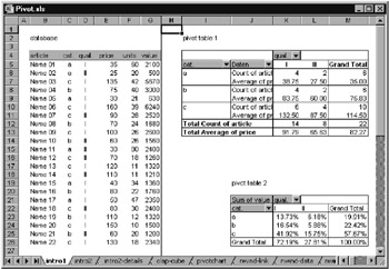
Figure 13-3: A database with two pivot tables

Pivot tables are created with the command DataPivottable and Pivotchart Report. This command summons the PivotTable wizard. The goal of this example (that is, pivot table 1 in Figure 13-3) is to determine for each product category and quality level the number of articles and their mean value. To accomplish this the following steps were executed:

Step 1 : Determines the origin of the data, which in the current example is the current worksheet.

Step 2 : Determines the range of cells containing the data: B4:G26. Step 3: Determines whether the pivot table is to be placed in the same worksheet or in a new one. As result there appears an empty matrix of a pivot table. At the same time the pivot toolbar is made visible, and the wizard disappears.

Step 4: Now it is time to move, with the mouse, data fields (column headers from the initial data) from the pivot table toolbar to their proper place in the table. See Figures 13.4 and 13.5. The two ranges "RowField" and "ColumnField" define the groups into which the table is to be divided. The range "DataField" specifies what information is to be displayed in the individual groups.

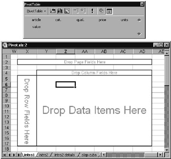
Figure 13-4: Above, the pivot table toolbar of Excel 2000; below, the new, still empty, pivot table

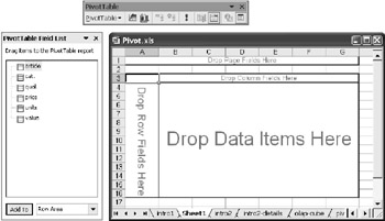
Figure 13-5: Above, the pivot table toolbar of Excel 2002; below, the new, still empty, pivot table

Begin with moving "cat." into the row field range, "qual." into the column field range, and "price" into the data field range. The result is the first pivot table, which looks like the table in Figure 13-6.

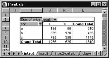
Figure 13-6: One step on the way to pivot table 1

In addition to the price, the number of articles is of interest, so drag the article field from the toolbar into the data range of the table (Figure 13-7).

Step 5: Figure 13-7 almost corresponds the requirements of the table. However, it is not the sum of the prices, but their mean that should be displayed. (Excel automatically calculates the sum for numerical data, and the number of items for text.) To display the means instead of the sums, place the cell pointer on a price field of the table (it doesn't matter which) and execute the command Field Settings. In the form that appears select the function Average and terminate the dialog. The result is that all the price fields are accommodated to the new function.

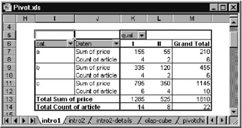
Figure 13-7: et another step

Step 6: Because averages are being computed, a number of decimal places are displayed, too many of which make the table unreadable. Therefore, open Field Settings once again, click on the button labeled Number, and select a new number format. In contrast to formatting with FormatCells, the new format holds not just for the selected cell, but for all the price cells.

Example 2

The purpose of pivot table 2, shown in Figure 13-3, is to calculate the value of the total contents of the warehouse. What percentage of the warehouse's value is tied up in a particular combination of product category and quality level? We proceed as follows :

Steps 1, 2, and 3 : Data source as above. (You can specify pivot table 1 as the data source, which is based on the same data.)

Step 4 : Drag "cat." into the row field range, "qual." into the column field range, and "value" to the data field range.

Step 5: Excel automatically creates sum fields for "value." This is correct in itself, but the results should be formatted as percentages. Therefore, invoke, using the pivot table toolbar, the Field Settings dialog for the value field. The button Options expands the dialog box. There you can indicate that the data are to be displayed as "% of total." (See Figure 13-8.)

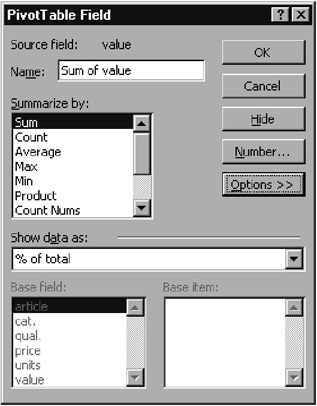
Figure 13-8: Representing a sum as a percentage of the total

Layout Options

Table Layout

Excel provides three grouping ranges for pivot tables: rows, columns , and sheets. At least one of these three group ranges must be taken up with a data field, so that a pivot table can be created in the first place. The simplest case is usually (as in the example above) that the column and row fields each contain a data field, as a result of which one has a "classic" data table in matrix form.

If several data fields are inserted into the row or column range, then Excel creates subcolumns or subrows and enlarges the table with subtotals. This makes the table more difficult to read, but it makes possible the creation of arbitrarily complex groupings into categories.

Greater clarity can be achieved by using one or more page ranges: With these are displayed list selection boxes above the actual pivot table, as we have seen in the case of the autofilter command. With these list selection boxes a single category can be selected; the pivot table is then reduced by this category. Additionally, the list selection field offers the possibility of displaying all categories simultaneously .

With the command FormatAutoformat the visual presentation of the pivot table can be completely changed. Excel offers in this respect a variety of predefined format combinations.

Layout Dialog

In Excel 97 the main structure of a pivot table could be changed only in step 3 of the pivot table wizard. The new pivot table toolbar is perhaps more intuitive to use, but on the other hand, you may nonetheless experience some nostalgia for the old dialog, which was often easier to use with very large pivot tables. It still exists: Summon the pivot table wizard (this works for an existing pivot table) and click in step 3 on the button Layout. The dialog pictured in Figure 13-9 then appears.

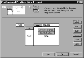
Figure 13-9: Dialog for altering the layout of a pivot table

Changing Pivot Tables After the Fact

There are almost endless ways of changing existing pivot tables. (The number of variants often causes some degree of confusion. Take a half hour to do some experimentation so that you become familiar with the most important operations.)

As soon as you move the cell pointer into a pivot table the pivot table toolbar should automatically appear. (If it does not, then you must activate the toolbar with ViewToolbars.) The most important command in the toolbar is Refreshdata. With this the indicated data are calculated afresh. The command must be executed when the source data have been changed, because Excel does not automatically recalculate pivot tables (in contrast to its behavior with almost all of its other worksheet functions).

With the toolbar you can perform such tasks as extending the pivot table with additional categories and inserting additional data fields. Of course, you can also remove fields from the table to make it smaller.

Tip	When a pivot table contains several data fields, you can remove all of them from the table (field "data"). Often, you will wish to remove only a single data field and not all of them. To do this, click the arrow button and deactivate those fields that you wish to remove (Figure 13-10).

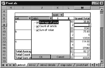
Figure 13-10: In the listbox individual fields can be deactivated.

Pivot table fields can be most easily reformatted with the pop-up menu command Field Settings. With the gray group fields the location (row, column, page) and number of subtotals can be set. In the case of data fields the type of calculation, display format, and number format can be defined (see below, under field settings ). Such changes affect all pivot table fields of the given group.

With the command DataSort the order of the data fields within the pivot table can be changed. The position of the cell pointer when the command is invoked determines the sort criterion.

Caution

Excel cannot change a pivot table to accommodate a fundamental change in the underlying data. For example, if you change the labels in your database and then wish to update the pivot table, Excel returns an error message and removes the changed columns from the table.

Field Settings

For formatting individual data fields Excel provides a number of rather complex options: With the pop-up menu command Field Settings or by double clicking on a data field (either in the table itself or in the layout dialog in step 3 of the pivot table wizard) you open the dialog box Pivottable Field, which reveals its complexity only after you have clicked on the Options button (see Figure 13-8).

The listbox Summarize By allows for the selection of one of a number of calculational functions and is self-explanatory. In the list Show Data As things are already becoming more complicated. The settings options can be divided into two groups:

CALCULATION PROCEEDS	AUTOMATICALLY
Normal:	Displays the actual numerical values.
% of total:	Displays data as a percentage of the grand total of all the data in the table.
% of row/column:	Displays data in each row or column as a percentage of the total for that row or column.
Index:	Shows values in relation to row and column totals using the following formula:
	(cell value total result) / (row total * column total)*

CALCULATION CONSIDERS	THE VALUE OF OTHER DATA FIELDS
Difference from:	Displays the data as the difference with respect to another item, specified by the base field and base item.
% Of:	Displays the data as a percentage of the value for the base field and base item.
% Difference From:	Displays the data as the difference from the specified value, but as a percentage difference.
Running Total In:	Unclear what this does. According to the documentation, it displays data as a running total.

For the last four named settings a second data field must be specified in relation to which the calculation is to proceed.

Grouping Results in Pivot Tables

The result lines in a pivot table can be grouped with the command DataGroup and OutlineGroup. This type of further processing of pivot tables is most useful with time- related data. Figure 13-11 presents an example.

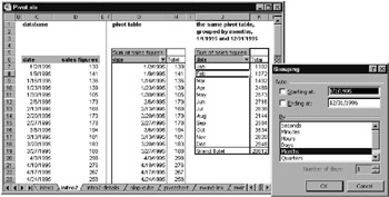
Figure 13-11: Sales figures for 1995 grouped by month

Tip

If, as in the above example, grouping is by month only, but the time period encompasses more than a year, Excel nonetheless forms only twelve groups. This means that the results for January comprise the results for all years in the time period, which is seldom a useful arrangement. The problem can be circumvented by specifying start and end dates explicitly in the Grouping dialog.

Another way of proceeding consists in grouping by year and another interval (months or quarters) simultaneously. Excel then constructs two principal groups (1995 and 1996) and within these groups, subgroups for each interval. Figure 13-12 shows an example of this, where the subsidiary grouping is for quarters instead of for months.

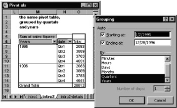
Figure 13-12: Grouping of sales figures by year and quarter

Tip

Excel is unable, for some reason that defies explanation, to group a data field if this is used as a page field of a pivot table (that is, in the region above the table). Fortunately, a solution is at hand: Drag the field into the column area, group it there, and then drag the resulting fields (year, quarter, etc.) back into the page area.

Drilldown and Rollup

Drilldown and rollup are the usual terms for the opening and closing of detailed results. There are two main options for this. The first consists in executing a double click for a cell in the grouping range. The result is that the affected group is made visible or invisible (Figure 13-13).

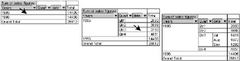
Figure 13-13: Making detailed results visible (drilldown)

On the other hand, if you execute a double click on a data field, Excel inserts one or more worksheets that contain the detailed results (Figure 13-14).

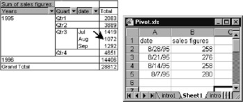
Figure 13-14: Sales figures for August 1996

Deleting Pivot Tables

There is no command for removing a pivot table from a worksheet. But that causes no difficulties: Simply select the entire range of cells and execute the command EditClearAll). With this the contents and the formatting of the cells will be deleted.

Pivot Tables for External Data

Pivot Tables can also be created for source data that do not reside in an Excel worksheet. The wizard accomplishes this in the first step with the command Multiple Consolidation Ranges or External Data Source.

If you select the option Multiple Consolidation Ranges, the pivot table wizard displays the appropriate dialog (see Chapter 11). With its assistance you can combine data from several Excel tables.

By an External Data Source is meant a database. When you select this option, Excel launches the auxiliary program MS Query to read in the data (see Chapter 12).

In each case the selected data are brought into Excel and stored there internally. The data are displayed as a pivot table. The raw data remain invisible.

Caution

The problem mentioned in the last chapter in connection with MS Query, that the names of Access databases are stored with the absolute pathname (with drive and directory), affects pivot tables as well.When both the Excel file and Access database file are moved into another directory, Excel no longer can find the source data and therefore cannot update the pivot table. A way out of this dilemma is presented later in this chapter.

Remarks

There are two principal ways of dealing with pivot tables with external data: The first consists in importing as much data as possible and then ordering it with the means available to pivot tables. This gives you maximal freedom in constructing the pivot table, but also requires a large amount of memory for storage. The other option is to attempt at the time of importation of the data to attempt to reduce this to a minimum. (This, then, costs more time in managing the often unwieldy MS Query.) The advantage is that the system requirements in Excel (processor demand, storage) are considerably less, and the processing speed correspondingly greater.

OLAP Cube Files

OLAP stands for Online Analytical Processing . By this is meant special methods for managing and analyzing multidimensional data. This again means data that are ordered according to several parameters. The Northwind table in Figure 13-15 presents a good example: Only two columns contain the actual data ( quantity and price ). All the other columns can be used as parameters or dimensions for grouping the data: order date, product category, country of the recipient, and so on. With every pivot table, then, you are ordering multidimensional data.

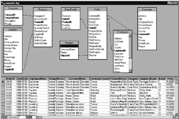
Figure 13-15: Development of a complex query with MS Query

Thus even though the Northwind database is through and through an example of multidimensional data, the notion of OLAP is usually used only when considerably more data are being analyzed (often gigabytes of data). Such databases are then called data warehouses . OLAP refers to the fact that the analytic functions can be executed quickly despite the huge volume of data, that is, online . For this a clever organization of data is necessary, and that is the particular feature of OLAP- capable database systems. (Such a system, which is particularly well optimized for the OLAP functions available from Microsoft, is, of course, Microsoft's own SQL server.

Let us return from this brief excursion into the wonderful world of OLAP to Excel. With pivot tables you can analyze not only traditional data sources (tables, relational databases), but OLAP data sources as well. MS Query provides the key. With this program you can access OLAP data sources directly. On the other hand, you can save the results of a database query ”even with respect to a relational database ”as a so-called OLAP cube.

Yet another new concept! A cube is a very general name for a multidimensional data set. An OLAP cube file with suffix *.cub makes it possible to store a static portrayal of a segment of the entire data set separate from the database. This offers a number of advantages: First, the cube file can be easily passed to another user . Second, the data are stored in a space-saving manner. Third, one can obtain very efficient access to these data. Of course, there are drawbacks: The organization of the data in the cube file is rigid (which limits the evaluation options). Moreover, changes in the source data (that is, in the database system) are not taken into account (that is, they can be accounted for only by rebuilding the cube file).

Even if you do not have access to a data warehouse , you can nonetheless try out the OLAP function. To do this, pose a query with MS Query that refers to a relational database (for example, as in Figure 13-15).

Now either you can specify in the last step of the query wizard that you wish to create an OLAP cube from this query, or you may execute in MS Query the command FILECREATE OLAP CUBE. In both cases the OLAP cube wizard appears (Figure 13-16). There you select in the first step the data fields (for example, sum of Quantity and sum of UnitPrice ). In the second step you specify the parameters of the data (for example, OrderDate , LastName of the Employees , CategoryName ). With time data you can also provide subcategories (year, quarter, month, etc.). In the third step you save the cube into another file.

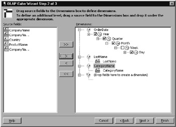
Figure 13-16: The OLAP cube wizard

Now you can create a pivot table in Excel based on this cube (Figure 13-17). In principle, this way of proceeding is the same as for the analysis of data that are available directly in Excel. But some details are different. For example, you cannot change the calculational function of the data fields (such as Sum ), since in the cube only the sum data are stored. If you now determine that you require the mean values, you must create the cube anew. What is new as well is that time series can be more easily evaluated (without the occasionally complicated Group command). But even here, time categories that you have not specified in the cube wizard are not available and cannot be reproduced with DataGroup.

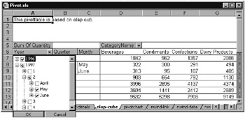
Figure 13-17: Pivot table based on an OLAP cube

When you exit the OLAP wizard, two files are saved in the directory Userdirectory\Application Data\Microsoft\Queries : The first is name1.oqy , with the SQL code of the OLAP query, and the other is name2.cub , with the results of the query. For the following example, olap.cub was stored in the same folder as the Excel file.

Tip	It is impossible to create a new pivot table on the basis of a *`.cub` file if the associated `.oqy`* file is absent.

Pointer

Among the Microsoft OLAP libraries can also be found ADOMD (that is, ADO multidimensional).With it you can access OLAP data sources as with the ADO library. There is insufficient space to go into this topic here.

A good introduction to the Microsoft OLAP world (with a chapter on ADOMD and a further chapter on Excel as OLAP analytical tool) is given in the book MS OLAP Services, by Gerhard Brosius.

Pivot Table Options

If you execute the command TABLE OPTIONS in the pivot table toolbar, the dialog shown in Figure 13-18 appears. The first block of options relates to formatting the pivot table. The significance of most of the options is clear, or else can be understood from the on-line help. (Click first on the question mark and then on the option in question.) It is often overlooked that in this dialog one can also give a new name to the pivot table. This is of particular practicality when you are managing several pivot tables in an Excel file.

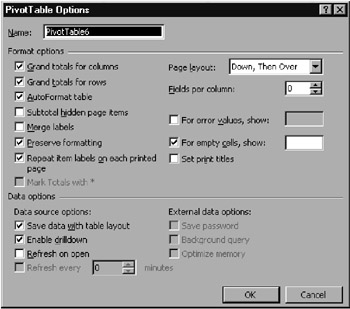
Figure 13-18: Pivot table options

The data options, on the other hand, require a bit more explanation. Save Data With Table Layoutx means that the query data are saved together with the Excel file. The advantage is that on next loading the data are immediately available. The disadvantage is that a large data set will bloat the Excel file. (The setting is relevant only when the data come from an external data source.)

Enable Drilldown relates to the behavior of the table following a double click. Normally, this will make visible or hide the detailed results. If this option is deactivated, Excel stops this behavior, which for pivot table novices is often confusing.

The Refresh options govern whether and when the basis data should be automatically updated. (In the default setting, updating takes place only when the corresponding command is explicitly executed.)

Background Query means that during updating of the data you can continue to work in Excel. This is above all interesting if access to an external database is relatively time-consuming .

The option Optimize Memory is, alas, only sketchily documented. Excel attempts in reading external data to proceed with minimal use of RAM. It is unclear how this is done and what disadvantages may accrue. (If there were no drawbacks, the option would be unnecessary.)

Pivot Charts

Pivot charts (see Figure 13-19) are something new in Excel 2000. These are charts that are directly connected to a pivot table. It is not possible to generate a pivot chart without an associated pivot table. Every change in the structure of the table leads to a change in the chart, and vice versa.

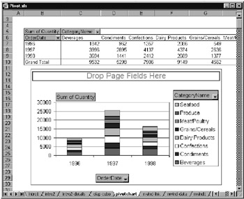
Figure 13-19: A pivot table with a pivot chart

To generate a new pivot chart execute the command DataPivottable and Pivotchart Report as you would for a new pivot table. In the first step of the pivot table wizard you specify that you wish to create a chart (not a table). The further steps are as before, though at the end both a table and chart are created (in a single sheet).

You can also equip an existing table with a pivot chart. Either start with the chart assistant (with the cell pointer in the pivot table or execute the command Pivotchart in the pivot toolbar.

Tip

Excel always generates a pivot chart in its own sheet. If you want to represent the chart next to or beneath the pivot table as an independent object, you must use a trick. Move the cell pointer outside the pivot table and launch the chart wizard. In step 2 specify the pivot table as data source. (Click on an arbitrary cell in the table.) In step 4 you now have available the option AS OBJECT IN WORKSHEET .