Section 6.4. Workarea

6.4. Workarea

All the logic is on the Workarea sheet . It is organized into functional areas using the same conventions as the other applications in the book. The overall layout is shown in Figure 6-10.

Figure 6-10. The organization of the Workarea sheet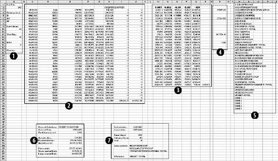

Item 1 in Column A contains named values used in other formulas. The area in Item 2 is used to hold the needed values from the Data sheet, based on the current settings. These values change when either the selected item or date changes.

Item 3 contains the regression model. The coefficients and intercept are at the top and are recalculated every time the data in Item 2 changes.

Item 4 uses the results of the regression calculations to set the control limits.

The data in Item 5 is used to populate the combo box that allows the user to select an item. The combo-box control requires a column as its input range. These values are headings on the Data sheet and are in a row. This area transposes them into a column.

Item 6 is a display area. It is used for the main display sheet and contains general information about the current item and date.

Item 7 is also a display area and is used by the system status report.

The first area (Item 1), used for named values, is detailed in Figure 6-11.

Figure 6-11. The section of Workarea indicated by Item 1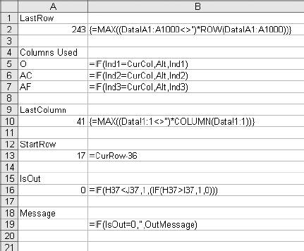

6.4.1. LastRow

The value in cell A2 is named LastRow. It keeps up with how many rows are used on the Data sheet. It is necessary to have a formula to calculate this because the number of rows could change if new data is put on the sheet. The formula is:

 {=MAX((DATA!A1:A1000) * ROW(DATA!A1:A1000))}

This array formula is covered in Chapter 3. As written, it only considers rows 11000. Since each row contains one day's data, this means the application can hold over two years of information. The formula can be changed to look at 5,000 rows by changing A1000 to A5000 in the formula. It has to be changed in both places and reentered using Crtl-Shift-Enter.

6.4.2. Columns Used

These values tell the model which column to use as independent variables . These formulas are necessary because they decide if the alternate needs to be used. The basic formula is:

 =IF(Ind1=CurCol,Alt,Ind1)

CurCol is a named value containing the column of the item being monitored. Here it is being tested against the first independent (Ind1). If they are equal the alternate value (Alt) is substituted. This formula is used for all three independents. The results in the range A5:A7 are named UsedInd1, UsedInd2, and UsedInd3.

6.4.3. LastColumn

The next value is LastColumn. It is the same as LastRow, except it looks at which columns are used.

6.4.4. StartRow

The model requires 35 days of data. Therefore, we need to pull data starting 36 days before the selected date, allowing one additional row for the headings. The named value StartRow in cell A13 keeps up with this value.

6.4.5. IsOut

The value IsOut in cell A16 is always 0 or 1. A 1 means the current item is out of the control limits. The formula is:

 =IF(H37<J37,1,(IF(H37>I37,1,0)))

H37 is the current actual value. J37 is the lower control limit and I37 is the upper control limit. Message in A19 is used on the Display sheet as shown in Figure 6-12.

Figure 6-12. The message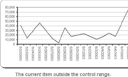

On the Display sheet, cell E28 contains this formula:

 =Message

The font for this cell is formatted red and bold. The message is blank if the item is inside the control limits and is set to outmessage if the item is outside the limits.

6.4.6. The Data Area

The next part of the Workarea sheet manages the link to the Data sheet, and is shown in Figure 6-13.

Figure 6-13. The section of Workarea indicated by Item 2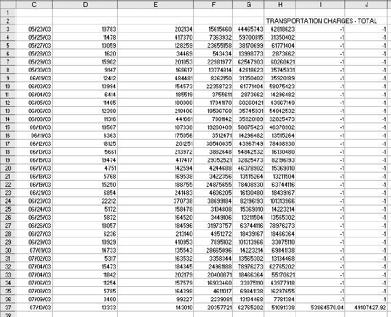

This is a holding area for data. It uses the settings to determine what data is needed and builds an area for the regression model to use. The last two columns of this area are used by the chart on the Display sheet.

The formula in C3 is:

 =TEXT(INDIRECT("Data!A"& ROW(A2)+StartRow),"mm/dd/yy")

Column A on the Data sheet contains the dates. The data starts in row two, as there are headings. The formula uses the named value StartRow to determine what row to start with. The formula fills down to C37. The dates are not used in the regression model, but they appear on the charts and in the displays. Excel's chart feature will fill in any skipped dates, and in this case we do not want that to happen. In the sample data we only have five days each week, so we don't need the other two days on the chart. The TEXT function is used to convert the date to a text string. This keeps Excel from seeing these as dates.

Columns D, E, and F are similar. They contain the independent variables . The basic formula in D3 is:

 =INDIRECT("data!" & UsedInd1 & ROW(A2)+StartRow)

Here we do not know the column in advance. It is determined by the named value UsedInd1. Cells E3 and F3 are the same but reference UsedInd2 and UsedInd3. These also fill down to row 37.

Columns G and H both contain the current data item. Column G is offset by one lag and is used in the regression calculations. Column H is not offset and is the dependent or Y variable. The formulas for these rows are:

 =INDIRECT("data!" & CurCol & StartRow+ROW(A2)-Lag) =INDIRECT("data!" & CurCol & ROW(A2)+StartRow) 

The heading in cell H2 uses the same formula except the heading is always in row 1. So, the formula is:

 =INDIRECT("data!" & CurCol & ROW(A1))

Columns I and J are used to put the control limits on the chart. These appear as small tick marks at the right end of the plot area, as shown in Figure 6-14.

Figure 6-14. The chart shows the control limits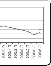

All the cells in these columns except the last row have a value of -1. The vertical axis of the chart is formatted with a minimum value of 0, as shown in Figure 6-15.

This keeps all the values except the last row off the chart. The values in row 37 are the control limits. Cell I37 has this formula:

 =Q37+T12

Cell Q37 is the current prediction and T12 has the allowable error. So, this is the upper control limit. In cell J37 the formula is:

 =MAX(Q37-T12,0)

This sets the lower limit. In some cases the limit would be a negative number, and for this kind of data that is not sensible. Therefore, we use a formula that will return a value of 0 if the limit comes out negative.

On the chart both of these items are formatted with no line, as shown in Figure 6-16.

Figure 6-15. Formatting the vertical axis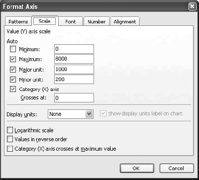

Figure 6-16. Formatting the control limits series on the chart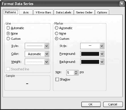

This makes the control limits appear as markers at the end of the chart.

6.4.7. The Regression Area

The regression area is shown in Figure 6-17.

Figure 6-17. The regression area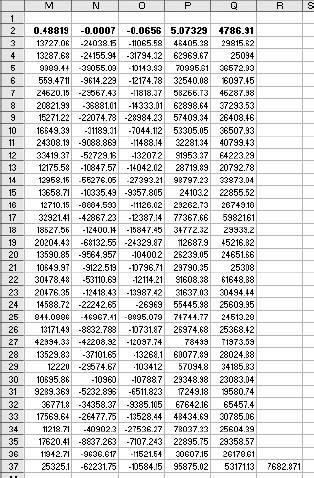

The coefficients and intercept are in row 2 and are calculated using this formula:

 {=LINEST(H3:H36,D3:G36,TRUE,FALSE)}

It is entered as an array formula in the range M2:Q2. The first parameter is the dependent or Y range. In this case it is the actual values in column H. We do not include row 37 because that is the day being checked. We run the regression using only days in the past.

The range D3:G36 contains the independent variables we looked at earlier. The third parameter (TRUE) tells the LINEST function not to force the intercept to be 0. The final parameter tells LINEST not to return the regression statistics. We are not doing analysis here. We just want the answer.

In cell M3 the formula is:

 =M$2*G3

This fills down but not to the right. Inconveniently, the LINEST function returns the coefficients in reverse order. So, the formulas have to be entered separately for each column. Column N has:

 =N$2*F3

And so on. Finally in column Q we add the intercept with this formula:

 =SUM(M3:P3,Q$2)

This is the predicted value.

The day being monitored is in row 37, and we need to know how accurate the prediction is. The formula in cell R37 is:

 =ABS(Q37-H37)

We use the absolute value because we need to know how much error there is, not the error itself. This results in a one-tailed distribution, which is easy to handle with Excel's statistical functions.

The results of the regression are used to set the control limits. This is done in the area shown in Figure 6-18.

Figure 6-18. The control limits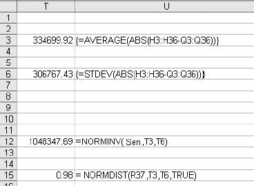

The actual values are in column H and the predictions are in Q. The array formula in cell T3 returns the average of the absolute values of the differences between the predicted and the actual. Once again, we do not use row 37 because it is the current day. We use an array formula for this because otherwise we would need another column with absolute error for the model.

In cell T6 we do the same thing in calculating the standard deviations of the errors.

These values are used in cell T12 to determine how much error is allowed for row 37. We know the mean and standard deviations of the errors, and we assume they are normally distributed. We know how much error we are willing to accept. Given these parameters, the NORMDIST function returns the value that is our limit. This is the amount of error that will cause an item to be flagged as an anomaly.

If an item is flagged, we need to know how far out it is. This is not just the size of the error. Very few predictions will be exactly right, and some error is expected. But relatively large errors should be rare. If we set the application's sensitivity to 0.99, we will be alerted when there is only a 1% chance that an item's error would occur as part of the past population of errors.

The formula in cell A15 calculates what percentage of errors is less than the error for the item being tested. If the formula returns a value of 0.98, then 98% of errors are less than the one for the item being tested.

6.4.8. The Combo Box Data Area

Column W of the Workarea sheet contains the names of the data items as shown in Figure 6-19.

Figure 6-19. The item names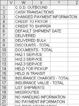

These are the headings from the Data sheet. The combo box control cannot use the headings directly because they are not in a column. The formula in cell W1 is:

 =IF(INDEX(Data!B$1:IV$1,1,ROW(A1))=0,"",INDEX(Data!B$1:IV$1,1,ROW(A1)))

It fills down to cell W255. This formula contains an IF function because the index function returns a value of zero if the referenced cell is empty. This would cause the combo box to display a long list of zeros after the last item name. The IF function returns a blank (=" ") if the referenced cell is empty, causing the combo box to display a blank for the unused columns.

6.4.9. The Main Display Area

There are two display areas on the Workarea sheet. Figure 6-20 has the first.

Figure 6-20. The display area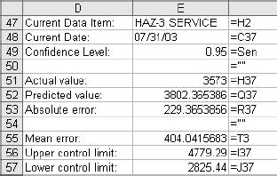

This area is named Display. The main display uses it for the information above the chart. All the values come from the Workarea sheet itself. The references are shown in the figure. The Display sheet references this range with an array formula applied to an area with the same number of rows and columns, as demonstrated in Figure 6-21.

Figure 6-21. The display sheet references an area on the Workarea sheet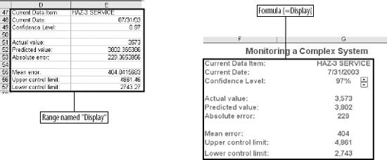

As in all the applications, this keeps the logic out of the display and allows the Display sheet to be concerned only with presentation issues.

The system status report is set up the same way, but some of its values come from the Data sheet. The formulas in its range on Workarea are shown in Figure 6-22.

Figure 6-22. Building the system status report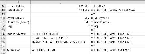

The earliest date that the application can test is in the 44th row because the model requires 43 days of history. The latest date is the last used cell in column A on the Data sheet. Figure 6-23 shows the range named "Stats," which contains this information, and its relationship with the systems status report.

Figure 6-23. The relationship between the Workarea and the system status report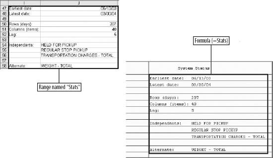

Again, the main point is keeping the logic and the presentation separate.